Chapter 11 The importance of variation

11.1 Learning objectives
By the end of this chapter, you will be able to:
- Appreciate why we need to measure variation as well as average effects of an intervention
- Understand the terms “standard deviation” and “confidence interval”
A note of warning: Chapter 11 to Chapter 14 are the most challenging in the book, insofar as they introduce several statistical concepts that are frequently misunderstood. We have minimized the amount of mathematical material in these chapters, and provide brief verbal summaries of the main points. Readers without a statistical background may find it helpful to try some of the exercises with interactive websites recommended in Check Your Understanding sections to gain a more intuitive understanding of the concepts covered here.
11.2 The importance of variability
When we are considering the impact of an intervention, we tend to focus on means: in particular on the difference in average outcomes between an intervention group and a control group. But what we are really interested in is variability - specifically, how much of the variability in people’s outcomes can be attributed to the intervention, and how much can be regarded as random noise. The widely-used method of analysis of variance gives us exactly that information, by looking at the total variability in outcomes, and considering what proportion is accounted for by the intervention.
To make this more concrete, consider the following scenario: You want to evaluate a weight loss program, Carbocut, which restricts carbohydrates. You compare 20 people on the Carbocut diet for 2 weeks with a control group where people are just told to stick to three meals a day (Program 3M). You find that those on Carbocut have lost an average of 1 lb more weight than those on 3M. Does that mean the diet worked? It’s hard to say just from the information provided: some people may think that the average loss is unimpressive; others may think that it is encouraging, especially over such a short time scale. These answers are about real-life significance of this amount of weight loss. But they disregard another issue: the statistical significance of the weight loss. That has nothing to do with meaningfulness in the real world, and everything to do with reproducibility of the result. And this relates to the variability of outcomes within each group.
11.2.1 Standard deviation
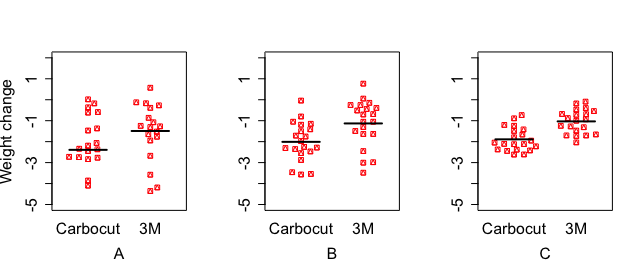
Consider Figure 11.1, which shows three different fictional studies. They have the same sample size in each group, 20. The mean difference in pounds of weight loss between the two diets (represented by the difference in the black horizontal lines) is similar in each case, but the variation within each group (the spread of points around the line) is greatest in scenario A, and least in scenario C. The intervention effect is far less impressive in scenario A, where 7/20 people in the Carbocut group score above the mean level of the 3M group, than in group C, where only 2/20 score above the 3M mean.
Figure 11.1: Simulated data from three studies comparing two diets. Each dot is the weight change of an individual. The horizontal bars show the group mean. Overlap between groups is greatest for study A and least for study C.
The spread in scores within each group is typically measured by the standard deviation, which is a mathematical way of representing how tightly bunched a set of scores is around the mean. If we want to know how solid a result is, in terms of how likely it would be to reproduce in a new study, we need to consider not just the mean, but also the standard deviation of the intervention effect. This website (https://www.mathsisfun.com/data/standard-deviation.html) explains how the standard deviation is computed, but in general, we can rely on statistics programs to do the calculations for us.
Why does the standard deviation matter? This is because, as noted above, the statistical significance of a finding, which indexes how likely a finding is to be reproducible in future studies, considers all the variation in scores, and looks at variation between groups relative to the variation within each group.
11.2.2 Confidence intervals
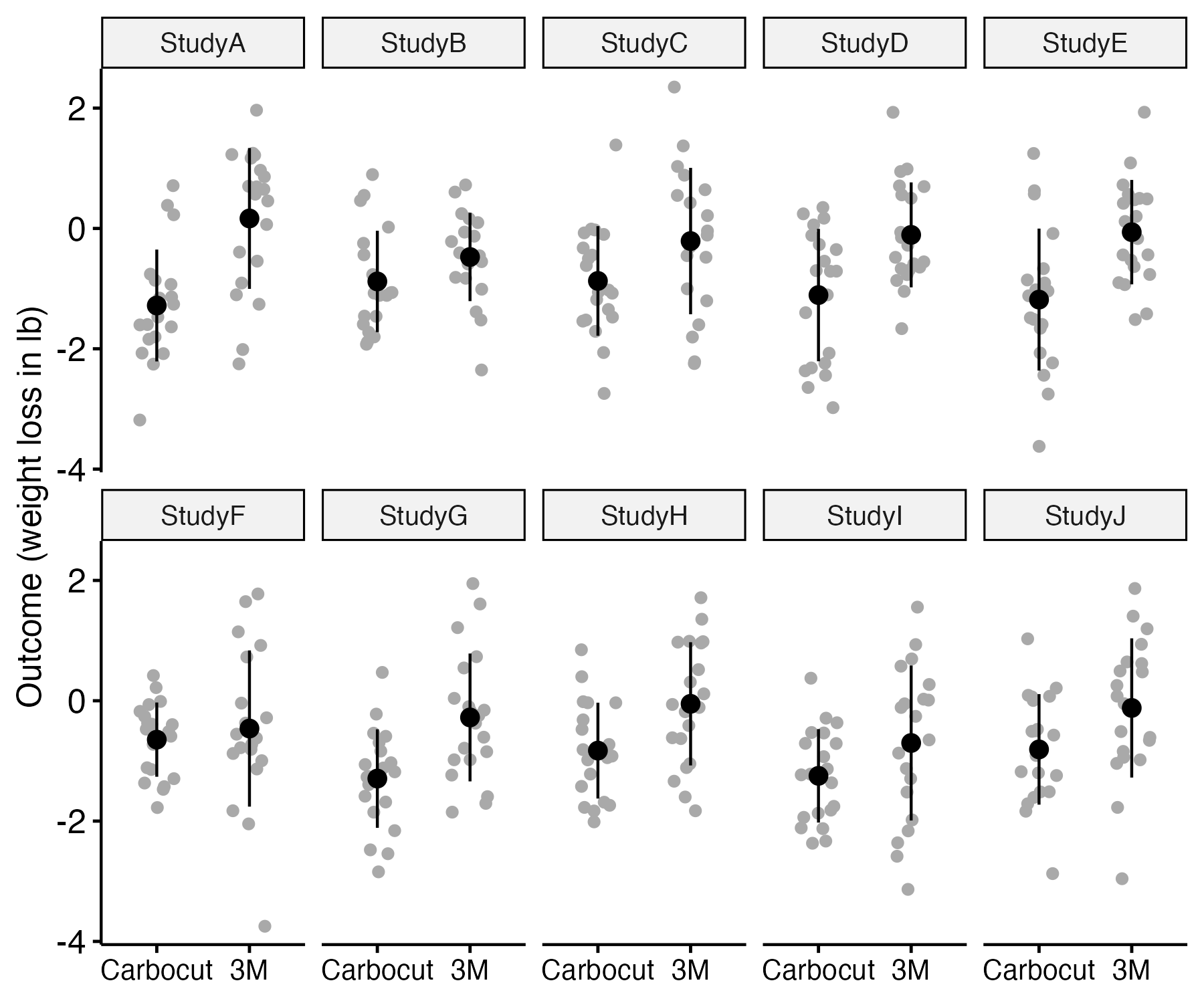
The confidence interval provides an index reflecting the precision of our estimate of the group difference. Suppose we were to run ten identical studies comparing the two diets, keeping the sample size the same each time. Figure 11.2 shows some simulated data of this scenario. In each case, the data were drawn by sampling from a population where the mean weight loss for Carbocut was 1 lb, and the mean loss for 3M was 0.25 lb. In both groups, the standard deviation was set to one. You may be surprised to see that the difference in means of the two groups fluctuates quite markedly, being substantial in study A, and negligible in study F, with other studies intermediate. The same computer code was used to generate the three plots: the different results are just random fluctuations due to chance, which will occur when you use random number generators in simulations. This relates to the topic of sampling, which we will cover in Chapter 13. The main take-home message is that when we run a study and get a mean difference between groups, this is an estimate of the true effect, which will contain some random noise.

Figure 11.2: Simulated data from ten studies comparing two diets. The observed mean is shown as a black point, and the SD as the black fins
When we report results from a study, we can report a confidence interval (CI) around the estimated mean difference between groups, which gives an indication of the uncertainty associated with the estimate; this will depend on the standard deviation and the sample size, both of which feature in its calculation.

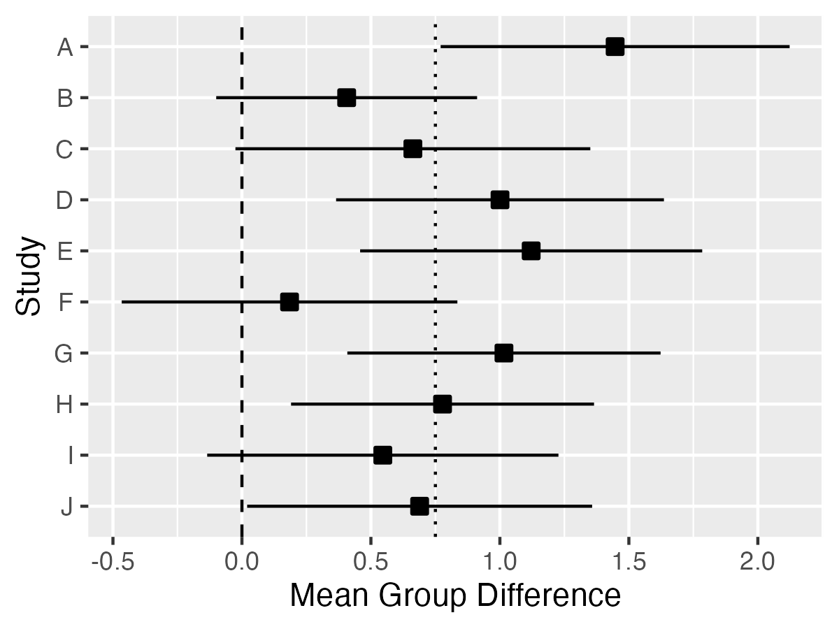
Figure 11.3: Mean difference (black square) with 95 per cent Confidence Intervals (fins) for 10 studies from previous Figure. Dashed line shows zero; dotted line shows true population difference
Figure 11.3 shows the mean group differences with 95% confidence intervals for the 10 studies from Figure 11.2. Because these data were simulated, we know that the true mean difference is 0.75, shown as a dotted vertical line, and can see that the mean estimates from the ten studies generally cluster around that value, but with a fair bit of variation. As we shall see in Chapter 13, high variation characterises studies with small sample sizes: the confidence intervals would be much smaller if we had 200 participants per group rather than 20. The dashed vertical line denotes zero. If the confidence interval includes zero, the study will fail to reach statistical significance on a t-test, which is a method of analysis that we will explain in Chapter 12. We can see that studies B, C, F and I would all be non-significant on this criterion. We will discuss in Chapter 13 how it is that we can get nonsignificant results even if there is a true group difference - and how to avoid this situation.
Reporting of confidence intervals
Those who set standards for reporting clinical trial results generally encourage researchers to include confidence intervals as well as means. Reporting of confidence intervals is useful, not least because it encourages researchers and readers of research to appreciate that the results obtained from a study are just estimates of the true effect, and there may be a wide margin of uncertainty around results from small samples. Some have pushed back against reporting of confidence intervals, either because of conceptual objections and/or because the confidence interval is widely misunderstood. The correct interpretation of a 95 per cent confidence interval is that if you conducted your study over and over again, on 95 per cent of occasions the confidence interval that you get will contain the true population mean. Illustrating this point, in Figure 11.3, you can see that for most studies, the confidence interval contains the true value, .75, but there is one study, study A, where there is a very large difference between means and the confidence interval does not include the true value.
11.3 Check your understanding
- Look at this website: https://shiny.rit.albany.edu/stat/confidence/, which has a simple interface that allows you to see how confidence intervals change as you vary the sample size and confidence level. First, check whether you understand what is shown on the plot. Can you predict what will happen if you:
- Increase the number in the Sample Size box?
- Change the Confidence Level?
- Change the Standard Deviation?
Try playing with the app by altering numbers in the boxes to see if your predictions are confirmed.