7 Extended Linear Regression: Practical 17
This practical extends the simple linear regression from the last practical to the context of multiple regression. While it is usually desirable to commence any analysis looking at the relationships between individual variables, often we want to look at how a particular outcome is affected by multiple variables. This is usually undertaken for to distinct reasons:
To fit a predictive model. For example, if recovery time from an operative procedure can be shown to depend on a group of variables which can be measured prior to the time of the operation, then it might be possible to predict which patients have a poor prognosis and to consider an alternative therapy for them.
To fit a causal model. We may be interested in the effect of changes in a single exposure variable on the outcome variable, but nevertheless recognise that the outcome may also be affected by changes in other variables. For example, as part of a study looking at whether haemoglobin level (Hb) or haematocrit (PCV) are risk factors for death due to ischaemic heart disease, a strong correlation was found between Hb and PCV and also between Hb and age. Was the relationship between Hb and PCV only apparent because they both increase with age or are they still related when age is taken into account? In other words, can we account for the confounding by age? We can view age as a common cause of Hb and PCV that we wish to control for to get at the true relationship between the exposure and outcome variables.
This practical is based on data from women aged 15-49 years from a rural area of The Gambia. One of the aims of the study was to look at factors affecting depression in these women. A series of questions were asked and a depression score was derived from the answers. The score can take any value between 0 (indicating no depression) up to 24 (indicating severe depression).
The factors which might affect depression in this dataset are: a) The number of living children the woman has. In this area, where a woman’s status is thought largely to depend on her fertility, the hypothesis was that depression would be associated with lower numbers of children. b) Prolapse (on clinical examination). Another hypothesis was that this common condition, which is rarely diagnosed and treated in this community, might be associated with depression.
The dataset is called depress.dta and the variables are as follows: * age : Single years; range 15 to 49 years * depscore : Depression score; range 0 to 24 * children : Number of living children; range 0 to 11 * any_prolapse : Whether woman had a prolapse; 0 = normal, 1 = prolapse seen on examination * type_prolapse : Type of prolapse a woman had; 0 = none, 1 = moderate, 2 = severe
We commence in the usual way by loading libraries, setting options, and reading in data.
#--- Load libraries
library(epiDisplay)
library(foreign)
library(psych)
library(magrittr)
library(tidyverse)

#--- Change to show no scientific notation & round to 3 decimal places
options(scipen = 10, digits=3)

#--- Set the plot theme to come out in black and white
theme_set(theme_bw())

#--- Read in the file
depress <- read.dta("./depress.dta", convert.factors = T)
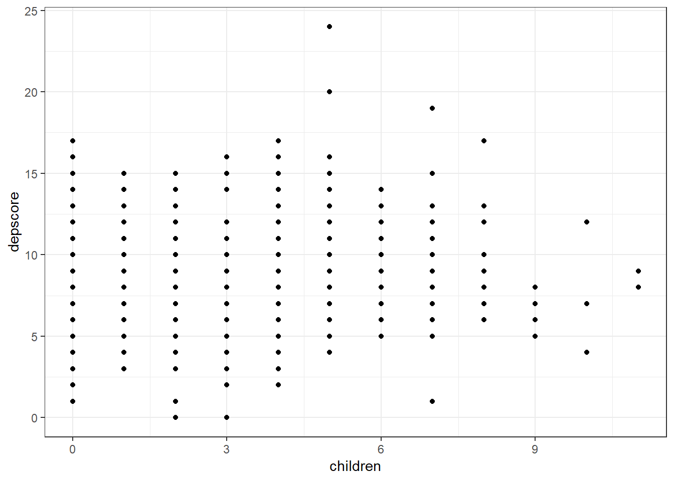
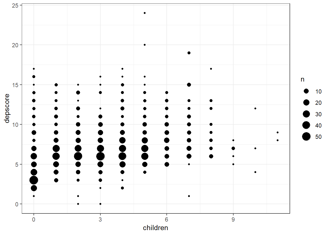
We first create a quick scatterplot and run a simple linear regression to look at the relationship between depression and the number of children a woman has. A so called bubble plot perhaps better displays this relationship - the size of the bubble is proportional to the number of individuals with that particular combination of x and y values.
#--- Plot depression score with scatterplot
depress %>% ggplot(aes(x = children, y = depscore)) + geom_point()
#--- Plot depression score with bubble plot
depress %>% ggplot(aes(x = children, y = depscore)) + geom_count()
#--- Run linear regression
mod1 <- depress %>% lm(depscore ~ children, data = .)
summary(mod1)
##
## Call:
## lm(formula = depscore ~ children, data = .)
##
## Residuals:
## Min 1Q Median 3Q Max
## -7.634 -1.868 -0.485 1.048 16.132
##
## Coefficients:
## Estimate Std. Error t value Pr(>|t|)
## (Intercept) 5.9518 0.1443 41.3 <2e-16 ***
## children 0.3832 0.0373 10.3 <2e-16 ***
## ---
## Signif. codes: 0 '***' 0.001 '**' 0.01 '*' 0.05 '.' 0.1 ' ' 1
##
## Residual standard error: 2.82 on 1065 degrees of freedom
## Multiple R-squared: 0.0901, Adjusted R-squared: 0.0892
## F-statistic: 105 on 1 and 1065 DF, p-value: <2e-16confint(mod1)## 2.5 % 97.5 %
## (Intercept) 5.67 6.235
## children 0.31 0.456