3.14 Non-Parametric Tests
Non-parametric (or distribution-free) tests do not assume that the distributions being compared are normal, so are useful alternatives where the assumptions of normality do not hold. They are called “non-parametric tests” because they do not estimate parameters for a model using a normal (or any other) distribution. Below there are two examples of these kinds of test along with the output you can expect.
3.14.1 Wilcoxon rank sum test
The ‘Wilcoxon Rank Sum test’ (also called ‘Mann-Whitney test’), is a distribution-free alternative to the t-test, and is used to test the hypothesis that the distributions in the two groups have the same median. For this test you will need to use the BABNEW.DTA dataset - we read in that dataset below.
Note that babnew appears in the Environment pane alongside bab9 - so we can readily access both datasets at once, no need to use an equivalent to Stata’s replace. This is the tradeoff for typing the dataset name each time. Note that it is possible to do away with much of the typing the dataset name by working in the tidyverse, or alternatively using attach(dataset) and then detach(dataset). This latter option is not recommended, as it can easily get confusing! Use short dataset names and let RStudio do the autocomplete work for you!
We also supply the code for the test and additional code to get the median by gender as it is not clear from the test which median is the higher median. The code to get the median comes from the tidyverse functions. We first pipe babnew into the group_by() function, which does exactly what it says on the tin: perform the following functions in groups defined by gender. We then use the summarise() function to extract a particular measure, that is, the median. We specify we want the summarise() function from dplyr in particular by prefixing the function with dplyr:: - the vcdExtra package also contains a function called summarise() and depending on the order in which the packages are loaded, one will mask the other - this is why we load the tidyverse last.
#--- Read in the file
babnew <- read.dta("./BABNEW.dta", convert.factors = T)

#--- Run the WMW test
babnew %$% wilcox.test(bweight ~ sex)
##
## Wilcoxon rank sum test with continuity correction
##
## data: bweight by sex
## W = 60000, p-value = 0.0003
## alternative hypothesis: true location shift is not equal to 0#--- Get medians
babnew %>% group_by(sex) %>% dplyr::summarise(median(bweight))## # A tibble: 2 x 2
## sex `median(bweight)`
## <fct> <dbl>
## 1 male 3290
## 2 female 3120#--- Note that the code below does not work!
#--- This is because the second pipe is sending babnew grouped by sex into the first argument of the median function
#--- ?median shows us that the first argument median() expects is not a dataset but the variable to summarise!
# babnew %>% group_by(sex) %>% median(bweight)
# ?median3.14.2 Wilcoxon Signed Rank Test
The non-parametric equivalent of the t-test for matched pairs is the ‘Wilcoxon signed rank test’. We will do this on the nonparametric.dta dataset, which contains 15 pairs of skinfold measurements, with each pair being a skinfold measurement on a single individual by two observers A and B.
We want to test for a difference in the two observers, so we check the distribution of the outcome variable in each group (using histograms). We have seen this histogram code before, we have just changed the variable names and the bin size.
#--- Read in the file
nonpara <- read.dta("./NONPARAMETRIC.dta", convert.factors = T)

#--- Plot histograms
nonpara %>% ggplot(aes(x = sfa)) + geom_histogram(bins = 5)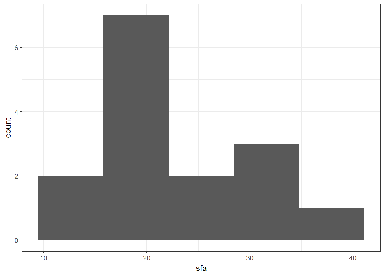
nonpara %>% ggplot(aes(x = sfb)) + geom_histogram(bins = 5)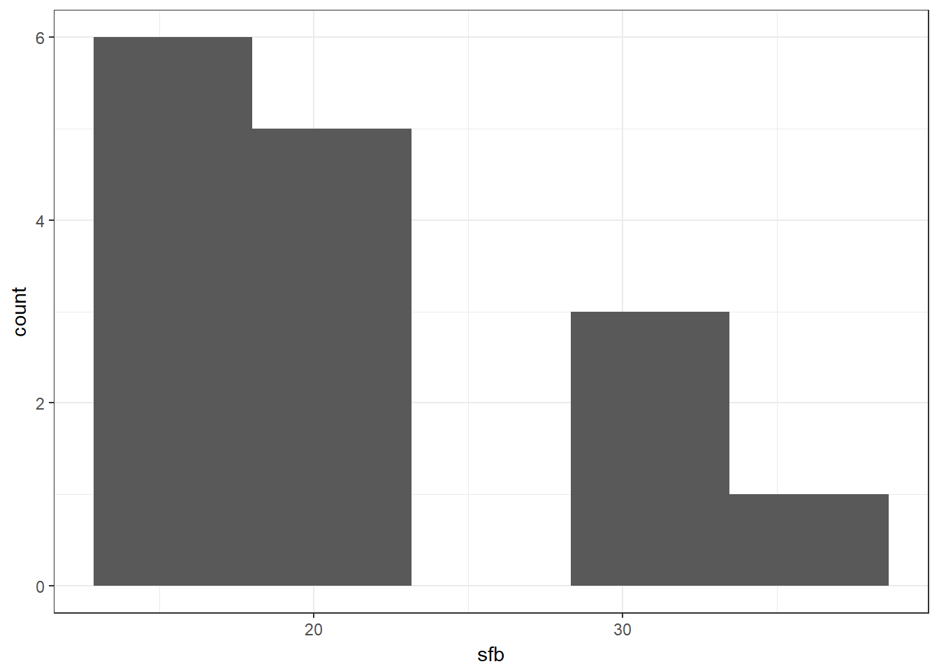
To plot both histograms at once and to run the test, we will need to reshape the data from wide to long. This is quite simple with the tidyverse function gather().
gather() goes from a ‘wide’ data format to a ‘long’ data format. Assuming multiple observations per individual, a wide data format is where each row is an individual, while a long data format is where each row is an observation. gather() uses the concept of key-value pairs. A key is a unique identifier (e.g. an observation or an individual) while a value (or values) are the values of a given set of data associated with the key. In this case, each skinfold observation is the key, and the values are the values of thoe measurements.
gather() takes as arguments: gather(data, name for new ‘key’ column, name for new ‘value’ column, first column where values are stored : last column where values are stored). The ‘:’ indicates include every column between the first and the last. The factor_key = T argument tells us to make the ‘key’ column a factor variable. Have a look at the nonpara dataset and compare it with the nonpara.l dataset to work out what we have done by using gather() - all the same data is there, it is just arranged slightly differently.
We see some new ggplot arguments in geom_histogram(). The alpha argument tells ggplot to put some transparency on the bars, and the position = “identity” argument tells ggplot to plot the histograms overlapping rather than stacked on top of one another.
#--- Convert from wide to long
nonpara.l <- nonpara %>% gather(observer, skinfold, sfa:sfb, factor_key=TRUE)

#--- Plot on the same histogram
nonpara.l %>% ggplot(aes(x = skinfold, fill = observer)) +
  geom_histogram(bins = 5, alpha = 0.5, position = "identity")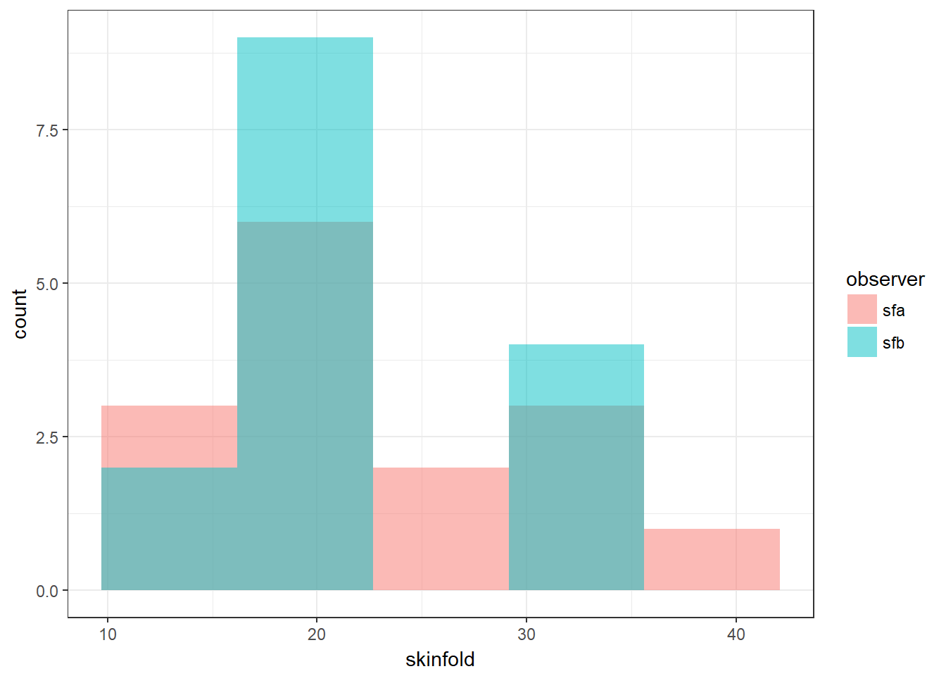
We now run the test and find strong evidence against the null hypothesis that the median skinfold value does not differ by observer.
#--- Run the Rank-Sum test
nonpara.l %$% wilcox.test(skinfold ~ observer, paired = T)
##
## Wilcoxon signed rank test with continuity correction
##
## data: skinfold by observer
## V = 100, p-value = 0.005
## alternative hypothesis: true location shift is not equal to 0Exercise 9.7: Run the equivalent t test using the paired = T option. What do you conclude?