4.3 Trends in proportions

Since birthweight is known to increase with length of gestation, we will use this fact to test for a linear trend in proportions. Gestational age was measured to the nearest week.

Let’s examine the histogram for gestational age.

#--- Plot gestational age
bab9 %>% ggplot(aes(x = gestwks)) + geom_histogram()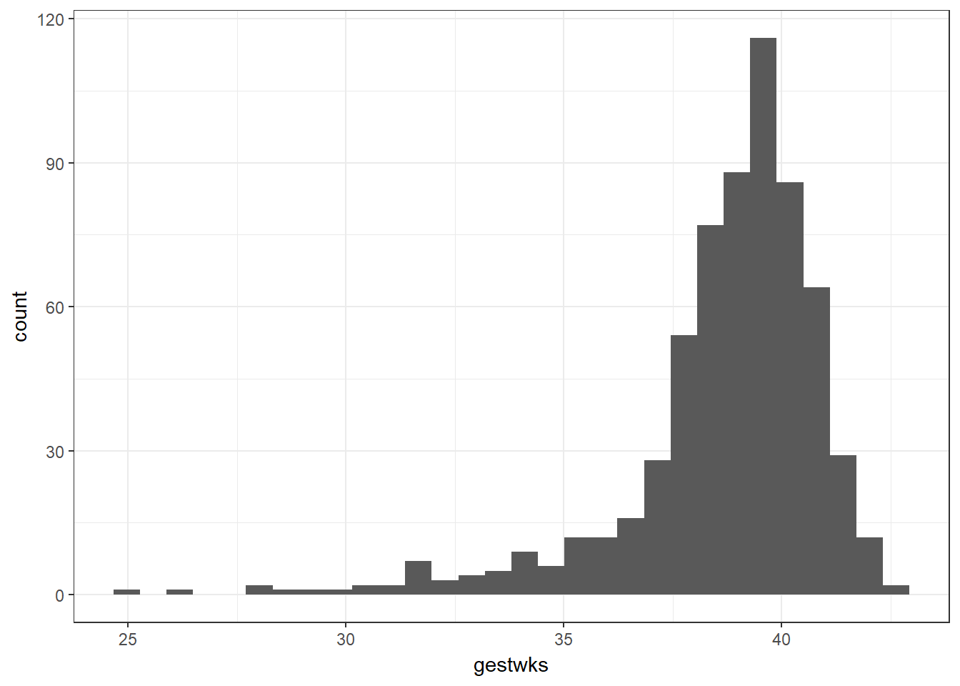

We notice that here we have left skew. This means that if we categorised the data by dividing gestwks into equally spaced groups of time (i.e. groups of 3.5 weeks) we would end up with unequal groups. So instead, we put an equal number of individuals into each group using the ntile() command and convert it to a factor. ntile() takes two arguments: the variable to divide into ntiles, and the number of ntiles desired.

The describeBy() command from the psych package gives a number of summary statistics for gestwks by values of gest5.

We can also get a 2x2 table from cc() in EpiDisplay.

#--- Get the quintiles
bab9$gest5 <- as.factor(ntile(bab9$gestwks, 5))

summary(bab9$gest5)

##   1   2   3   4   5 
## 129 128 128 128 128

#--- Extract the top of each quintile by finding the maximum (and thus the cut points)
bab9 %>% group_by(gest5) %>% dplyr::summarise(max(gestwks))

## # A tibble: 5 x 2
##   gest5 `max(gestwks)`
##   <fct>          <dbl>
## 1 1               37.7
## 2 2               38.7
## 3 3               39.5
## 4 4               40.3
## 5 5               42.3

#--- Examine gestational age by quintile
bab9 %$% describeBy(gestwks, gest5)

## 
##  Descriptive statistics by group 
## group: 1
##    vars   n mean   sd median trimmed  mad  min  max range  skew kurtosis
## X1    1 129 35.1 2.63     36    35.6 1.91 24.7 37.7    13 -1.49     2.12
##      se
## X1 0.23
## -------------------------------------------------------- 
## group: 2
##    vars   n mean   sd median trimmed  mad  min  max range  skew kurtosis
## X1    1 128 38.3 0.32   38.3    38.3 0.43 37.7 38.7     1 -0.12    -1.31
##      se
## X1 0.03
## -------------------------------------------------------- 
## group: 3
##    vars   n mean   sd median trimmed  mad  min  max range  skew kurtosis
## X1    1 128 39.2 0.21   39.1    39.2 0.25 38.8 39.5  0.69 -0.18     -1.2
##      se
## X1 0.02
## -------------------------------------------------------- 
## group: 4
##    vars   n mean   sd median trimmed  mad  min  max range  skew kurtosis
## X1    1 128 39.9 0.24   39.9    39.9 0.34 39.5 40.4  0.84 -0.04    -1.27
##      se
## X1 0.02
## -------------------------------------------------------- 
## group: 5
##    vars   n mean  sd median trimmed  mad  min  max range skew kurtosis
## X1    1 128   41 0.5   40.8    40.9 0.44 40.4 42.4     2 1.01     0.18
##      se
## X1 0.04

#--- Table for low birthweight and gestational age
bab9 %$% cc(lbw, gest5, graph= F)

## 
##                 gest5
## lbw              1  2     3      4      5   
##   low            65 10    2      3      0   
##   normal         64 118   126    125    128 
##                                             
##   Odds ratio     1  11.86 63.08  41.75  Inf 
##   lower 95% CI      5.58  15.89  12.88  32.4
##   upper 95% CI      27.73 547.99 215.46 Inf 
## 
## Chi-squared = 217 , 4 d.f., P value = 0 
## Fisher's exact test (2-sided) P value = 0