3.2 Descriptive Statistics
We first look at the first few rows of the dataset.
R’s summary output differs from Stata. We use the summary() function to examine a variable; this is equivalent to the summ function in Stata. To get the equivalent to summ, detail we can use the describe() function in the psych package.
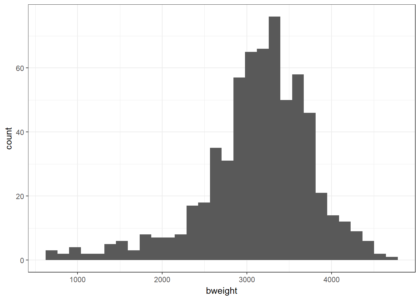
We can quickly graphically look at the distribution of a variable using the hist() command. Let’s take a look at the bweight variable. Because R is capable of storing more than one dataset in its working memory, we have to tell R both the dataset (bab9) and the variable (bweight) that we are interested in. We do this by using a dollar sign - the dollar sign says from the dataset on the left, extract the variable on the right.
#--- Investigate the first few rows of the dataset
head(bab9)
## id matage ht gestwks sex bweight matagegp gestcat
## 1 1 33 no 37.7 female 2410 2 2
## 2 2 34 no 39.2 female 2977 2 2
## 3 3 34 no 35.7 female 2100 2 1
## 4 4 30 no 39.3 male 3270 2 2
## 5 5 35 no 38.4 female 2620 3 2
## 6 6 37 no 37.9 male 3260 3 2#--- Get summary statistics
summary(bab9)## id matage ht gestwks sex
## Min. : 1 Min. :23 no :552 Min. :24.7 male :326
## 1st Qu.:161 1st Qu.:31 yes: 89 1st Qu.:38.0 female:315
## Median :321 Median :34 Median :39.2
## Mean :321 Mean :34 Mean :38.7
## 3rd Qu.:481 3rd Qu.:37 3rd Qu.:40.2
## Max. :641 Max. :43 Max. :42.3
## bweight matagegp gestcat
## Min. : 630 Min. :1.00 Min. :1.00
## 1st Qu.:2850 1st Qu.:2.00 1st Qu.:2.00
## Median :3200 Median :2.00 Median :2.00
## Mean :3129 Mean :2.38 Mean :1.86
## 3rd Qu.:3550 3rd Qu.:3.00 3rd Qu.:2.00
## Max. :4650 Max. :4.00 Max. :2.00#--- Get detailed summary statistics
describe(bab9)## vars n mean sd median trimmed mad min max range
## id 1 641 321.00 185.19 321.0 321.00 237.22 1.0 641.0 640.0
## matage 2 641 33.97 3.87 34.0 34.10 4.45 23.0 43.0 20.0
## ht* 3 641 1.14 0.35 1.0 1.05 0.00 1.0 2.0 1.0
## gestwks 4 641 38.69 2.33 39.1 39.04 1.48 24.7 42.4 17.7
## sex* 5 641 1.49 0.50 1.0 1.49 0.00 1.0 2.0 1.0
## bweight 6 641 3129.14 652.78 3200.0 3181.91 518.91 630.0 4650.0 4020.0
## matagegp 7 641 2.38 0.81 2.0 2.40 1.48 1.0 4.0 3.0
## gestcat 8 641 1.86 0.35 2.0 1.95 0.00 1.0 2.0 1.0
## skew kurtosis se
## id 0.00 -1.21 7.31
## matage -0.27 -0.48 0.15
## ht* 2.08 2.35 0.01
## gestwks -2.05 6.19 0.09
## sex* 0.03 -2.00 0.02
## bweight -0.96 1.78 25.78
## matagegp -0.09 -0.58 0.03
## gestcat -2.08 2.35 0.01#--- Plot birthweight
hist(bab9$bweight)
We now use the sapply() command to check the class of each variable in the data. The sapply() function iterates over each column of the dataset of interest and performs the given function, in this case, class(). In other words, sapply() is a way of performing the same action to each variable of the dataset. class() tells us what data type each of our variables is.
We pipe the dataset of interest into the sapply() command. Piping is fundamental to tidy R code. A standard pipe looks like %>%. You can insert a pipe with Ctrl-Shift-M. The pipe takes whatever is on the left of it and then uses it as the first argument of the function on the right. You can see below two equivalent ways of coding the sapply() command. Pipes are useful as they allow you to chain together multiple different functions. While in this case, the piping seems to have made little functional difference, its utility will become clear in future practicals as the coding becomes more complex.
We see from our sapply() explorations that matagegp & gestcat have been read in as numeric (i.e. numbers), but they should be what R calls factor variables. Factor variables are R’s way of representing categorical variables. We convert them to factors using the as.factor() command and assign this new factor variable to the old numeric variable, overwriting it in the process.
#--- Check the class of each variable
bab9 %>% sapply(class)
## id matage ht gestwks sex bweight matagegp
## "numeric" "numeric" "factor" "numeric" "factor" "numeric" "numeric"
## gestcat
## "numeric"#--- Same code without a pipe:
# sapply(bab9, class)
#--- Convert factors
bab9$matagegp <- as.factor(bab9$matagegp)
bab9$gestcat <- as.factor(bab9$gestcat)