Chapter 1 Consolidation of MATH1055

1.1 Random Variables

Consider a random experiment, that is, some well-defined repeatable procedure that produces an observable outcome which could not be perfectly predicted. Rolling a die, measuring daily rainfall in a region or the number of goals scored in a football match are all examples of random experiments.

A random variable represents a number, the value of which depends on the outcome of some underlying random experiment.

The following are both examples of random variables:

Let $X$ be the number of heads observed when tossing a fair coin three times.
Let $X$ be the lifespan of a Playstation.

Note that random variables can take a finite or countable number of discrete values (number of heads), or be continuous (length of time).

Random variables are often described mathematically using functions known as the probability mass function or the probability density function. These functions describe the probabilities of the outcome of a random variable.

Let $X$ be a discrete random variable. The function $p_X$ such that \[p_X(x) = P(X=x)\] is called the probability mass function (PMF) of $X$.

A PMF is a probability measure for the outcomes of the discrete random variable $X$. Commonly the PMF of a random variable is represented by a histogram: plot $p_X(x)$ against $x$.

Let $X$ be the number of heads observed when tossing a fair coin three times. Calculate the PMF of $X$.

The complete set of possible outcomes when flipping the coin three times is:

\[\big\{ HHH, \, HHT, \, HTH, \, HTT, \, THH, \, THT, \, TTH, \, TTT \big\}.\]

Each possible outcome occurs with probability $\frac{1}{8}$. There is one possibility ($TTT$) with zero heads obtained, three possibilities ($HTT, \, THT, \, TTH$) with one head obtained, three possibilities ($HHT, \, HTH, \, THH$) with two heads obtained, and one possibility ($HHH$) with three heads obtained. Therefore the PMF of $X$ is given by

\[ p_X(x) = \begin{cases} 1/8, & \text{if $x=0$}, \\[3pt] 3/8, & \text{if $x=1$}, \\[3pt] 3/8, & \text{if $x=2$}, \\[3pt] 1/8, & \text{if $x=3$}, \\[3pt] 0, & \text{otherwise.} \end{cases}\]

The histogram of this PMF is plotted below.

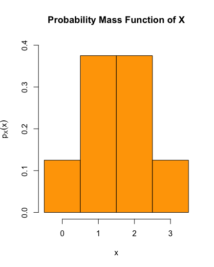
The R code for the PMF histogram (ignoring some customisation) appearing in the solution of Example 1.1.4 is:

x = c(0,1,1,1,2,2,2,3)
brks = c(-0.5,0.5,1.5,2.5,3.5)
hist(x, breaks=brks, probability=TRUE, col="orange", ylim = c(0,0.4))

Let $X$ be a continuous random variable. The function $f_X$ such that for any interval $I \subset \mathbb{R}$, \[\int_I f_X(x) dx = P(X \in I),\] if indeed such a function exists, is called the probability density function (PDF) of $X$.

Commonly the PDF of a random variable is represented by a curve: plot $f_X(x)$ against $x$.

The life span $X$ of a Playstation is distributed by the PDF \[f_X(x)= \begin{cases} 7e^{-7t}, & \text{if } x\geq 0, \\ 0,& \text{if } x< 0. \end{cases}\] Plot the PDF of $X$ in the region $x>0$, and calculate the probability that the Playstation breaks within a two year warranty.

Plotting the PDF of X, that is, plotting $f_X(x)$ against $x$ when $x>0$, obtain:

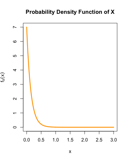
Applying Definition 1.1.5, calculate \[\begin{align*} P \big( 0 \leq X \leq 2 \big) &= \int_0^2 f_{X}(x) \,dx \\[3pt] &= \int_0^2 7e^{-7x} \,dx \\[3pt] &= \left[ -e^{-7x} \right]_0^2 \\[3pt] &= -e^{-14} + e^0 \\[3pt] &= 1 - e^{-14}. \end{align*}\]

The R code for the PDF plot appearing in the solution of Example 1.1.6, with some customisation removed, is:

x = seq(0,3,0.01)
y = 7* exp(-7*x)
plot(x, y, type = "l", col="orange", lwd=3)

The PDF of a continuous random variable is completely analogous to the PMF of a discrete random variable.

Alternatively to the PMF or the PDF, one can describe a random variable using the cumulative distribution function.

Let $X$ be a random variable. The function $F_X$ such that \[F_X(x) = P(X \leq x)\] is called the cumulative distribution function (CDF) of $X$.

Note the CDF is defined for both discrete and continuous random variables.

It is also worth noting that a CDF will only output values that lie between $0$ and $1$. This makes intuitive sense since the function output represents a probability. This is also the case for the PMF of a discrete random variable.

It is not the case that a PDF must take values between $0$ and $1$ as illustrated by Example 1.1.6. Why?

The CDF satisfies further useful identities pertaining to probabilities for the value of the random variable $X$:

$P(X>x) = 1 - F_X(x)$;
$P(x_1 < X \leq x_2) = F_X(x_2) - F_X(x_1)$.

Consider the random variable $X$ describing the number of heads observed when tossing a fair coin three times from Example 1.1.4. Calculate the CDF of $X$.

We have

for $x<0$ that $P(X \leq x) = 0$;
for $0 \leq x<1$ that $P(X \leq x) = P(X=0) = \frac{1}{8}$;
for $1 \leq x<2$ that $P(X \leq x) = P(X=0) + P(X=1) = \frac{1}{8} + \frac{3}{8} = \frac{1}{2}$;
for $2 \leq x<3$ that $P(X \leq x) = P(X=0) + P(X=1) + P(X=2) = \frac{1}{8} + \frac{3}{8} + \frac{3}{8} = \frac{7}{8}$;
for $x>3$ that $P(X \leq x) = P(X=0) + P(X=1) + P(X=2) + P(X=3) = \frac{1}{8} + \frac{3}{8} + \frac{3}{8} + \frac{1}{8} =1$.

Therefore the CDF of $X$ is given by

\[ F_X(x) = \begin{cases} 0, & \text{if $x<0$}, \\[3pt] 1/8, & \text{if $0 \leq x<1$}, \\[3pt] 1/2, & \text{if $1 \leq x<2$}, \\[3pt] 7/8, & \text{if $2 \leq x<3$}, \\[3pt] 1, & \text{if $x \geq 3$.} \end{cases}\]

Consider the random variable $X$ describing the lifespan of a Playstation from Example 1.1.6. Calculate the CDF of $X$

We want to calculate the function $F_{X}(x)$ such that $F_{X}(x) = P(X \leq x)$. Taking $I=(-\infty,x]$ in Definition 1.1.5, we have that \[F_X(x) = P(X \leq x) = \int_{-\infty}^{x} f_X(u) \,du.\] Here $u$ is a dummy variable: we have already used $x$ to describe the input of $F_{X}$ and since this features as an integral bound in the final expression, we relabel the input of $f_X$ to $u$.

If $x<0$, since $f_X(u)=0$ for all $u<x$, and so it follows that $F_{X}(x)=0$. Assume $x\geq0$, then \[\begin{align*} F_X(x) &= P(X \leq x) \\[3pt] &= \int_{-\infty}^{x} f_X(u) \,du \\[3pt] &= \int_0^x 7e^{-7u} \,du \\[3pt] &= \left[ -e^{-7u} \right]_0^x \\[3pt] &= -e^{-7x} + e^{0} \\[3pt] &= 1-e^{-7x}. \end{align*}\]

Therefore \[F_{X}(x) = \begin{cases} 1-e^{-7x}, & \text{if } x\geq 0, \\[3pt] 0, & \text{if } x<0. \end{cases}\]

Both of these examples highlight identities allowing us to calculate the CDF of a random variable $X$ from the PMF/PDF: \[ F_X(x) = P(X \leq x) = \begin{cases} \sum\limits_{x_i \leq x} p_X(x_i), & \text{if $X$ is discrete,} \\[9pt] \int_{-\infty}^x f_X(u) \,du, & \text{if $X$ is continuous.} \end{cases} \]

The following result allows us to additionally move from the CDF to the PDF of a continuous random variable.

If $F_X(x)$ is the CDF of a continuous random variable $X$, then the PDF of $X$ is given by \[f_X(x) = \frac{d F_X(x)}{dx}.\]

Consider the random variable $X$ governing the lifespan of a Playstation from Example 1.1.6. Verify that the PDF $f_X(x)$ (see Example 1.1.6) and the CDF $F_X(x)$ (see solution to Example 1.1.9 ) satisfy the identity of Lemma 1.1.10.

1.2 Discrete Distributions

There are a number of discrete probability distributions with which we should be familiar. All distributions discussed in this section can be studied further via the following application.

For each discrete distribution in the dropdown menu, the app allows you to choose values for parameters of the distribution in the Inputs window. The probability mass function of the distribution with the specified parameters is plotted. This allows for the study of the behavior of the PMF as each parameter varies.

The Inputs window also allows for a sample size to be chosen. The app will simulate taking this many samples from the chosen distribution. These samples are then displayed via a histogram plot in the window Simulation Plot, and in some cases a frequency table. It can be observed that as the sample size increase, the simulated histogram more closely resembles the PMF of the chosen distribution.

Discrete Uniform Distribution

Let $a$ be an integer, and $b$ be a positive integer. Suppose $X$ is randomly chosen from the integers in the list \[a,a+1, a+2, \ldots, a+b\]

where each number has an equal probability of being selected. Then $X$ is a random variable known as the discrete uniform distribution, denoted $U(a,b)$. Specifically \[p_{X}(x) = \frac{1}{b+1}, \qquad \text{for } x =a, a+1, \ldots, a+b.\]

One can calculate that

$\mathbb{E} [X] = a + \frac{b}{2}$;
$\text{Var}(X) = \frac{1}{12} b (b+2)$.

Rolling a dice is an example of a discrete uniform random variable with $a=1$ and $b=5$.

Bernoulli Distribution

Consider a random experiment which either results in a success or a failure. We denote a success by $1$, and a failure by $0$. The probability of success is given by a value $p \in [0,1]$, and so the probability of failure is $1-p$. This experiment can be described by a random variable $X$ where \[p_{X}(x) = \begin{cases} p, & \text{for } x =1, \\ 1-p, & \text{for } x=0. \end{cases}\] $X$ is known as a Bernoulli distribution.

One can calculate that

$\mathbb{E} [X] = p$;
$\text{Var}(X) = p(1-p)$.

Whether or not a client decides to enter a business deal after an initial meeting could be modeled as a Bernoulli distribution.

The following R code can be used to find 10 samples taken from a Bernoulli distribution with $p=0.7$.

library(Rlab)
rbern(10,0.7)

The following code evaluates the PMF of a Bernoulli distribution with $p=0.7$ at $x=0$.

library(Rlab)
dbern(0,0.7)

Binomial Distribution

Let $n$ be an integer greater than $1$. Consider $n$ Bernoulli trials that are all independent, and each one has the same chance of success $p$. Let $X$ be a random variable denoting the total number of successes across all $n$ Bernoulli trials. $X$ can take any integer value $k$ among $0,1,\ldots,n$. What is the probability that $X$ takes some fixed value of $k$?

Any particular sequence that contains exactly $k$ successes (each success happening with probability $p$) will also contain $n-k$ failures (each failure happening with probability $(1-p)$). So the sequence has probability $p^k (1-p)^{n-k}$ of happening. There are ${n \choose k}$ sequences with $k$ successes, and so the probability that $X=k$ is ${n \choose k} p^k (1-p)^{n-k}$. Specifically

\[p_{X}(k) = {n \choose k} p^k (1-p)^{n-k}, \qquad \text{for } k =0,1,\ldots n.\]

$X$ is called a Binomial distribution and is denoted $\text{Bin}(n,p)$.

One can calculate that

$\mathbb{E} [X] = np$;
$\text{Var}(X) = np(1-p)$.

The number of clients who decide to enter a business deal after an initial meeting with a group of $n$ clients could be modeled as a Binomial distribution.

The following R code can be used to find 10 samples taken from a Binomial distribution with $n=15$ and $p=0.7$.

rbinom(10,15,0.7)

The following code evaluates the PMF of a Binomial distribution with $n=15$ and $p=0.7$ at $x=11$.

dbinom(11,15,0.7)

Geometric Distribution

Consider an infinite sequence of Bernoulli trials that are all independent, and each one has the same chance of success $p$. Let $X$ be a random variable denoting the first Bernoulli trail that is a success. $X$ can take any positive integer value $1,2,3,\ldots$. For some fixed positive integer $k$, what is the probability that $X=k$?

For the $k^{th}$ trial to be the first success, one would require $k-1$ failures up to that point each with an independent probability of $1-p$. A subsequent success on the $k^{th}$ attempt happens with probability $p$. Therefore the probability that $X=k$ is $p(1-p)^{k-1}$. Specifically

\[p_{X}(k) = p (1-p)^{k-1}, \qquad \text{for } k =1,2,3,\ldots.\]

$X$ is called a geometric distribution, and is denoted $\text{Geom}(p)$.

One can calculate that

$\mathbb{E} [X] = \frac{1}{p}$;
$\text{Var}(X) = \frac{1-p}{p^2}$.

Note that the smaller $p$ is, the longer one has to wait for a success on average.

The number of happy customers served before encountering an unhappy customer could be modeled via a geometric distribution.

The following R code can be used to find 10 samples taken from a geometric distribution with $p=0.3$.

rgeom(10,0.3)

The following code evaluates the PMF of a geometric distribution with $p=0.3$ at $k=3$.

dgeom(3,0.3)

Negative Binomial Distribution

Consider an infinite sequence of Bernoulli trials that are all independent, and each one has the same chance of success $p$. Let $X$ be a random variable denoting the number of Bernoulli trails undertaken to encounter $r$ successes. $X$ can take any positive integer value $r,r+1,r+2,\ldots$. For some fixed positive integer $k$, what is the probability that $X=k$?

For the $k^{th}$ trial to be the $r^{th}$ success, one would require $r-1$ successes and $(k-1)-(r-1) = k-r$ failures before the $k^{th}$ trial. Each of these successes has an independent probability of $p$, and each failure has an independent probability of $(1-p)$. There are ${k-1 \choose r-1}$ possible sequences consisting of $r-1$ successes and $k-r$ failure. The subsequent success on the $k^{th}$ attempt happens with probability $p$. Therefore the probability that $X=k$ is ${k-1 \choose r-1} p^k (1-p)^{k-r}$ Specifically

\[p_{X}(k) = {k-1 \choose r-1} p^k (1-p)^{k-r}, \qquad \text{for } k =r,r+1,r+2,\ldots.\]

$X$ is called a negative binomial distribution, and is denoted $\text{NegBin}(r,p)$.

One can calculate that

$\mathbb{E} [X] = \frac{r}{p}$;
$\text{Var}(X) = \frac{r(1-p)}{p^2}$.

Note that $\text{NegBin}(1,p) = \text{Geom}(p)$.

The number of parts manufactured before encountering $r$ defective parts could be modeled via a negative binomial distribution.

The following R code can be used to find 10 samples taken from a negative binomial distribution with $r=4$ and $p=0.3$.

rnbinom(10,4,0.3)

The following code evaluates the PMF of a negative binomial distribution with $r=4$ and $p=0.3$ at $k=8$.

dnbinom(8,4,0.3)

Poisson Distribution

Consider the number of occurrences of a certain event over a fixed time period, given there are $\lambda>0$ occurrences on average. The number of occurrences $X$ can be modeled by a Poisson distribution, denoted $\text{Po}(\lambda)$. The probability mass function of $X$ is

\[p_{X}(k) = e^{- \lambda} \frac{\lambda^k}{k!} , \qquad \text{for } k =0,1,2,\ldots.\]

One can calculate that

$\mathbb{E} [X] = \lambda$;
$\text{Var}(X) = \lambda$.

The number of hits on a website per day can be modeled with a Poisson distribution.

The following R code can be used to find 10 samples taken from a Poisson distribution with $\lambda=5$.

rpois(10,5)

The following code evaluates the PMF of a Poisson distribution with $\lambda=5$ at $k=3$.

dpois(3,5)

Hypergeometric Distribution

Consider a finite population of size $N$. Suppose $a$ of the population have some distinguishing feature, and the remaining $N-a$ do not. If $n$ of the population are chosen at random, let $X$ denote how many of the $n$ selected from the population have the distinguishing feature. $X$ is modeled by a hypergeometric distribution. The probability mass function of $X$ is

\[p_{X}(k) = \frac{{a \choose k}{N-a \choose n-k}}{{N \choose n}} , \qquad \text{for } k =\max(n+a-N,0),\max(n+a-N,0)+1,\ldots, \min(a,n).\] One can calculate that

$\mathbb{E} [X] = \frac{an}{N}$;
$\text{Var}(X) = \frac{an(N-a)(N-n)}{N^2 (N-1)}$.

A company supplies parts to a customer in large quantities. The customer deems the product acceptable if the proportion of faulty parts is kept suitably low. Instead of testing the entire batch, the customer tests a subset of the parts. This process could be modeled by a hypergeometric distribution.

1.3 Continuous Distributions

Additionally there are a number of continuous probability distributions with which we should be familiar. All distributions discussed in this section can be studied further via the following application.

For each continuous distribution in the dropdown menu, the app allows you to choose values for parameters of the distribution in the Inputs window. The probability density function of the distribution with the specified parameters is plotted. This allows for the study of the behavior of the PDF as each parameter varies.

The Inputs window also allows for a sample size to be chosen. The app will simulate taking this many samples from the chosen distribution. These samples are then displayed via a histogram plot in the window Simulation Plot. It can be observed that as the sample size increase, the simulated histogram more closely resembles the PMF of the chosen distribution.

Uniform Distribution

The continuous uniform distribution is a distribution that can take an infinite number of equally likely values. Specifically for a continuous uniform distribution $X$, denoted $U(a,b)$, the probability density function is given by \[f_X(x) = \begin{cases} \frac{1}{b-a}, & \text{for } a<x<b, \\[3pt] 0, & \text{otherwise}, \end{cases}\]

and the cumulative density function is given by \[F_X(x) = \begin{cases} 0, & \text{for } x\leq a, \\[3pt] \frac{x-a}{b-a}, & \text{for } a <x <b, \\[3pt] 1, & \text{otherwise}. \end{cases}\]

One can calculate that

$\mathbb{E} [X] = \frac{1}{2} (b+a)$;
$\text{Var}(X) = \frac{1}{12}(b-a)^2$.

The following R code can be used to find 10 samples taken from a continuous uniform distribution with $a=0$ and $b=1$.

runif(10,0,1)

The following code evaluates the PDF of a uniform distribution with $a=0$ and $b=1$ at $x=\frac{1}{3}$.

dunif(1/3,0,1)

Exponential Distribution

Consider the occurrences of some specific event, given there are $\lambda>0$ occurrences on average in some fixed time period. The time from now until the next event $X$ can be modeled by the exponential distribution, denoted $Exp(\lambda)$. Specifically the probability density function of $X$ is \[f_{X}(x) = \begin{cases} \lambda e^{-\lambda x}, & \text{if } x>0, \\[3pt] 0, & \text{if } x \leq 0, \end{cases}\]

and the cumulative density function is \[F_{X}(x) = \begin{cases} 1 - e^{- \lambda x}, & \text{if } x>0, \\[3pt] 0, & \text{if } x \leq 0. \end{cases}\]

One can calculate that

$\mathbb{E} [X] = \frac{1}{\lambda}$;
$\text{Var}(X) = \frac{1}{\lambda^2}$.

The time it takes for a cashier to process a customer could be modeled via an exponential distribution.

The exponential distribution is inherently linked to the Poisson distribution: the time between successive events in a Poisson distribution is modeled by the exponential distribution.

The following R code can be used to find 10 samples taken from an exponential distribution with $\lambda=2$.

rexp(10,2)

The following code evaluates the PDF of an exponential distribution with $\lambda=2$ at $x=\frac{2}{3}$.

dexp(2/3,2)

Gamma Distribution

Consider the occurrences of some specific event, given there are $\lambda>0$ occurrences on average in some fixed time period. The time $X$ from now until the event has occurred $n$ times can be modeled by the Gamma distribution, denoted $Gamma(n,\lambda)$. Specifically the probability density function of $X$ is \[f_{X}(x) = \begin{cases} \frac{\lambda^{n}}{(n-1)!} x^{n-1} e^{-\lambda x}, & \text{if } x>0, \\[3pt] 0, & \text{if } x \leq 0. \end{cases}\]

The definition of the gamma function can be generalised to $n$ being a real number, but this requires the use of the Gamma function $\Gamma(n)$.

One can calculate that

$\mathbb{E} [X] = \frac{n}{\lambda}$;
$\text{Var}(X) = \frac{n}{\lambda^2}$.

The time it takes for a cashier to process $n$ customer could be modeled via a Gamma distribution.

Note that setting $n=1$ recovers the exponential distribution from the Gamma distribution. Furthermore the Gamma distribution $Gamma(n,\lambda)$ is equal to the sum of $n$ independent Exponential distributions $Exp(\lambda)$.

The following R code can be used to find 10 samples taken from a gamma distribution with $\lambda=2$ and $n=5$.

rgamma(10,5,rate=2)

The following code evaluates the PDF of a gamma distribution with $\lambda=2$ and $n=5$ at $x=\frac{2}{3}$.

dgamma(2/3,5,rate=2)

Normal Distribution

Suppose one has a random variable $X$ that follows a distribution that has mean $\mu$, variance $\sigma^2$, mode $\mu$ and is symmetric about the mean. Then $X$ can be modeled by the normal distribution, which we denote by $N(\mu,\sigma^2)$. Specifically the probability density function of $X$ is \[f_{X}(x) = \frac{1}{\sqrt{2\pi} \sigma} e^{- \frac{(x-\mu)^2}{2\sigma^2}}.\]

One can verify from the probability density function that

$\mathbb{E} [X] = \mu$;
$\text{Var}(X) = \sigma^2$.

The cost of a piece of equipment sampled across different sellers could be modeled by a normal distribution.

The central limit theorem, seen in the upcoming Section 1.4, demonstrates why the normal distribution plays such an important role in probability and statistics.

The distribution $N(0,1)$ is known as the standard normal distribution. The probabilities $P \big( N(0,1) < a \big)$ for any $a \in \mathbb{R}$, denoted $\Phi_N(a)$, are commonly read from a z-table. Specifically, here $\Phi_N$ is the CDF of the standard normal distribution.

The following R code can be used to find 10 samples taken from a normal distribution with $\mu=2$ and $\sigma=1$.

rnorm(10,2,1)

The following code evaluates the PDF of a normal distribution with $\mu=2$ and $\sigma=1$ at $x=3$.

dnorm(3,2,1)

Chi-squared Distribution

Consider $n$ samples from a standard normal distribution. Let $X$ be the random variable describing the distribution of the sum of the squares of these samples. Then $X$ can be modeled by the Chi-squared distribution, denoted $\chi^{2}_n$.

One can calculate that

$\mathbb{E} [X] = n$;
$\text{Var}(X) = 2n$.

Expressing the probability distribution function or the cumulative distribution function of the chi-squared distribution requires the use of the Gamma function $\Gamma(n)$.

It can be shown that the Chi-squared distribution is a special case of the Gamma distribution: $\chi^{2}_n = Gamma \left(\frac{n}{2},2 \right)$.

The following R code can be used to find 10 samples taken from a chi-squared distribution with $n=7$.

rchisq(10,7)

The following code evaluates the PDF of a normal distribution with $n=7$ at $x=5$.

dchisq(5,7)

1.4 Central Limit Theorem

The Central Limit Theorem is a key result in probability theory that describes the distribution of the mean of a sample from any distribution.

Central Limit Theorem Let $X_1,X_2,\dots,X_n$ be independent and identically distributed (IID) with finite mean $\mu$ and variance $\sigma^2$. Let $S_n = X_1 + \cdots + X_n$. Then \[ \frac{S_n - n\mu}{\sigma \sqrt{n}} \longrightarrow N(0,1).\]

That is to say, for sufficiently large values of $n$, the sample mean $\bar{X} = \frac{S_n}{n}$ of $X_1, X_2, \ldots , X_n$ can be approximated by the normal distribution $N \left( \mu,\frac{\sigma}{\sqrt{n}} \right)$.

Crucially the Central Limit Theorem illustrates the natural importance of the normal distribution.

The following app explores the Central Limit Theorem. We are able to choose the distribution from which we take a sample from among three continuous example distributions. Furthermore we can pick the parameters within these distributions using the first slider. The PDF of the chosen theoretical distribution is shown in the first plot. The second slider determines the value $n$ in Theorem 1.4.1, that is, how many observations of the distribution are taken to calculate a sample mean. Finally the number of sample means calculated is controlled by the third slider. The second plot illustrates the theoretical distribution of the means, and a histogram of the sample means. Note this is always a normal distribution.

Let $X_1,X_2,\dots,X_{100}$ each be the time that it takes the cashier in Jimmys local cornershop to process each of the hundred customers who will come in today. On average the cashier serves a customer in a quarter of a minute. Let $S_{100}=X_1+\ldots + X_{100}$ be the total time it will take for all one hundred customers to be served, and $\bar{X}=\frac{S_{100}}{100}$ be the average time it takes to serve each of these $100$ customers. Find limits within which $\bar{X}$ will lie with probability $0.95$.

In Example 1.3.1, we saw that the time it takes a cashier to serve a customer can be modeled by an exponential distribution $Exp(\lambda)$. Therefore we can assume $X_1,X_2,\dots,X_{100}$ are IID exponential random variables. Now $\frac{1}{4} = \mathbb{E}[X_i] = \mathbb{E}[Exp(\lambda)] = \frac{1}{\lambda}$, so conclude $\lambda=4$, and hence $\text{Var}(X_i) = \frac{1}{16}$. Therefore, \[\begin{align*} E \left[ S_{100} \right] &= E \left[ \sum\limits_{i=1}^{100} X_{i} \right] \\[3pt] &= \sum\limits_{i=1}^{100} E[X_i] \\[3pt] &= 100 \cdot \frac{1}{4} \\[3pt] &= 25; \\[5pt] \end{align*}\] and \[\begin{align*} \text{Var}(S_{100}) &= \text{Var} \left( \sum\limits_{i=1}^{100} X_{i} \right) \\[3pt] &= \sum\limits_{i=1}^{100} \text{Var}(X_i) \\[3pt] &= 100 \cdot \frac{1}{16} \\[3pt] &= \frac{25}{4} \end{align*}\] where the second equality of the variance calculation has used independence of the $X_i$. It follows that

\[\begin{align*} E\left[\bar{X}\right] &= E\left[ \frac{S_{100}}{100} \right] \\[3pt] &= \frac{1}{100} E\left[ S_{100} \right] \\[3pt] &= \frac{1}{4} \end{align*}\] and \[\begin{align*} \text{Var}(\bar{X}) &= \text{Var} \left( \frac{S_{100}}{100} \right) \\[3pt] &= \frac{1}{100^2} \text{Var} \left( S_{100} \right) \\[3pt] &= \frac{1}{1600}. \end{align*}\]

Since $n=100$ is sufficiently large, by the Central Limit Theorem, $\bar{X}$ is approximately normally distributed. Specifically \[\frac{\bar{X}-\frac{1}{4}}{\sqrt{\frac{1}{1600}}} \approx N(0,1).\]

The question asks us to find $a,b$ such that $P(a < \bar{X} < b)=0.95$. Calculate

\[\begin{align*} 0.95 &= P(a < \bar{X} < b) \\[5pt] &= P \left( \frac{a-\frac{1}{4}}{\sqrt{\frac{1}{1600}}} < \frac{\bar{X}-\frac{1}{4}}{\sqrt{\frac{1}{1600}}} < \frac{b-\frac{1}{4}}{\sqrt{\frac{1}{1600}}} \right) \\[5pt] &\approx P \left( \frac{a-\frac{1}{4}}{\sqrt{\frac{1}{1600}}} < N(0,1) < \frac{b-\frac{1}{4}}{\sqrt{\frac{1}{1600}}} \right) \tag{*}. \end{align*}\]

However one also has that \[\begin{align*} 0.95 &= P \left( \Phi^{-1} (0.025) < N(0,1) < \Phi^{-1} (0.975) \right) \\[5pt] &= P \big( -1.96 < N(0,1) < 1.96 \big). \tag{**} \end{align*}\]

Equatating like-terms between equations ( * ) and ( ** ) gives

\[\begin{align*} \frac{a-\frac{1}{4}}{\sqrt{\frac{1}{1600}}} &= -1.96, \\[5pt] \frac{b-\frac{1}{4}}{\sqrt{\frac{1}{1600}}} &= 1.96. \end{align*}\]

Therefore,

\[\begin{align*} a &= 0.25 - 1.96 \cdot \frac{1}{40} = 0.201, \\[5pt] b &= 0.25 + 1.96 \cdot \frac{1}{40} = 0.299. \end{align*}\]

Probability Methods and Time Series

Probability Methods and Time Series

Chapter 1 Consolidation of MATH1055

1.1 Random Variables

1.2 Discrete Distributions

1.3 Continuous Distributions

1.4 Central Limit Theorem