Chapter 7 Time Series
Throughout our study of probability and statistics, we often look at random samples. You will be used to seeing:
\[\textit{Consider random variables } X_1, X_2, \ldots, X_n \\ \textit{ that are independent and identically distributed.}\]
Our strategy for modelling would then be to choose a standard distribution that we believe will fit the identical random variables well. Observations could be used to fit the probability model.
Consider a class of thirty Year 4 students. The students line up in a random order. Consider random variables \(X_1, X_2, \ldots, X_{30}\) where \(X_i\) is the height of the \(i^{th}\) student. Then \(X_1, X_2, \ldots, X_{30}\) are independent and identically distributed.
One might reasonably choose to model the random variables using a normal distribution, or perhaps a bimodal distribution to account for male and female students.
However in many real world scenarios, an assumption that such a collection of random variables are independent may clearly be inappropriate: random variables may intuitively correlate.
Consider the price of Bitcoin in pounds throughout the coming September: the price is described by random variables \(X_1,X_2,\ldots, X_{30}\), where \(X_i\) is the price at noon on the \(i^{th}\) of September.
Making a prediction about the price on \(30^{th}\) September would currently be difficult, however knowing the price on \(29^{th}\) September would allow for a more accurate prediction: \(X_{29}\) and \(X_{30}\) are not independent. Furthermore knowing all of \(X_1, \cdots, X_{29}\) would allow for a even more accurate prediction, we could study at the current trend in the price changes.
In this case, it would be inappropriate to fit a choice of standard distribution to observed data to model the random variables. We require another type of probabilistic model. The appropriate concept is time series.
7.1 Introduction to Time Series
Before defining time series, we recall the definition of a stochastic process.
A stochastic process is a family of random variables \(\left\{ X_t: t \in \mathcal{T} \right\}\) where the index \(t\) belongs to some parameter set \(\mathcal{T}\), and each of the random variables can take the same set of possible values. The possible values that the random variables can take is known as the state space.
We will only consider stochastic process where the parameter set \(\mathcal{T}\) is discrete, and the members of \(\mathcal{T}\) are equally spaced. For example, the positive integers \(\{ 0,1,2,3,\ldots \}\).
Let \(\{ X_t : t \in \mathcal{T} \}\) be a stochastic process. A time series is a set of observations of the stochastic process where each observation is recorded at a specific time \(t \in \mathcal{T}'\) for some subset \(\mathcal{T}'\) of \(\mathcal{T}\).
Typically the parameter set \(\mathcal{T}\) is representative of time, and a time series is therefore a collection of data observations made sequentially over time. Note there is no assumption in Definition 7.1.2 that the random variables \(X_t\), and therefore the observations, are independent.
The following datasets could be modeled using a time series:
Number of new COVID-19 cases per week in 2020;
Daily FTSE100 value over a given period;
Retail sales figures over successive weeks.
It is easy to think that one observed data point in any of these examples above is almost certainly not independent of nearby observations.
A time series can be represented graphically using a time plot, a line plot of the observations against time.
A dataset describing the number of hours of sunshine for the East Midlands region for each month during 2020 could be modeled with a time series. This time series can be represented graphically with a time plot:

A time plot is first step in an analysis of a time series and can highlight key features.
The R package tswge contains a number of time series datasets. You should install the package on your personal device. The library dfw.2011 contains data on monthly temperatures in Dallas from January 2011 to December 2020.
A time plot of this data can be created.
Note that the plot produced by the above code does not have a sensible labeling on the x-axis. Each point is labelled by its index as a data point, rather than by the relevant month and year. This can be corrected by converting the data to a ts object, an object designed for working with time series data.
library(tswge)
dfw.2011.ts = ts(dfw.2011,start=c(2011,1),frequency=12)
dfw.2011.ts
plot(dfw.2011.ts)Here frequency=12 indicates to the device that the time series data is monthly, and start=c(2011,1) indicates that the first data point was observed in January 2011. ts objects can be further studied in the relevant R documentation.
The seasonality of a time series refers to how observations may flucuate or change in a short cyclic period.
A dataset describing the quarterly passenger numbers from the Port of Dover in the years 2011-2021 could be modeled with a time series. This time series can be represented graphically with a time plot:
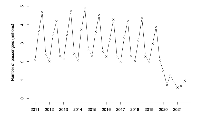
The time series exhibits seasonality: the passenger numbers are cyclical on a yearly basis. Passenger numbers increase from Q1 through Q2 of each year in the run-up to the summer, with numbers peaking in Q3 before decreasing again through Q4 to a low during the winter of the following Q1.
It is also worth noting that the time series does exhibit anomalous data during the years 2020 and 2021. There is an obvious explanation for this.
The trend of a time series refers to how observations may change in general in the long term.
A dataset describing the sales of Australian red wine in the years 1980-1995 could be modeled with a time series. This time series can be represented graphically with a time plot:
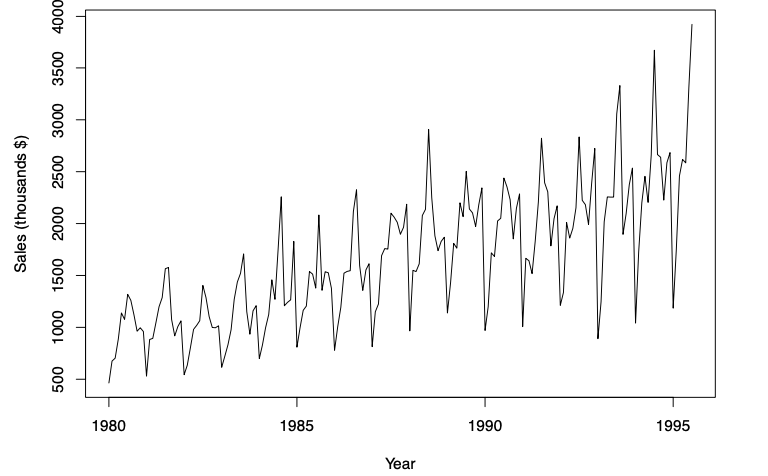
The time series exhibits some seasonality. However what is also notable is a positive trend: despite the cyclical fluctuations up and down, over time the sales are increasing. This can be observed in the higher highs and higher lows, or observed in that a line of best fit would have a positive gradiant.
It is also worth noting that the variability of the data is increasing with time: the distance between the highest and lowest sales number within a cycle increases each year.
7.2 Stationarity
As well as analysing trend and seasonality, it is worth discussing how the statistical properties of the random variables of a time series \(\{ X_t : t \in \mathbb{Z} \}\) change over time. Informally a times series is said to be stationary if the statistical properties do not change with time. The formal definition is as follows:
A time series \(\{ X_t : t \in \mathbb{Z} \}\) is stationary if
\(\mathbb{E}(X_t)\) is independent of \(t\);
\(\text{Var} (X_t) = \sigma^2 < \infty\) for all \(t\);
For all values of \(h\), the quantity \(\text{Cov} (X_t, X_{t+h})\) is independent of \(t\);
The first two criteria in this definition are clear. Time should not have an effect on the expectation or the variance of the observations made in the time series. The final criteria states that the covariance between \(X_t\) and \(X_{t+h}\) depends only on the number of time steps \(h\) between the two observations, not on the time step \(t\) at which the first observation is made.
In reality many time series are not stationary.
Consider the time series from Example 7.1.4 describing the number of hours of sunshine in the East Midlands during each month in 2020. Clearly this is not a stationary time series since the random variable governing sunshine hours in July will not have the same expectation as the random variable governing the sunshine hours in December.
Consider the time series from Example 7.1.6 describing the quarterly passenger numbers from the port of Dover in the years 2011-2021. This is not a stationary time series: the seasonality observed means that the expectation of a random variable corresponding to a Q1 will not be equal to the expectation of a random variable corresponding to a Q3.
Consider the time series from Example 7.1.8 describing the sales of Australian red wine in the years 1980-1995. The trend of increasing sales with time means that the expectation of the random variables also generally increases, that is to say, \(\mathbb{E}(X_t)\) is dependent on \(t\). Therefore the time series is not stationary.
As observed in these examples, seasonality or trend will result in a time series being non-stationary.
In many real-world applications, such as those above, only one realisation of the observations is possible. Without being able to simulate multiple time series observations it can be difficult to argue that the variance and covariance criteria of Definition 7.2.1 fail to hold. Indeed note in the three above examples we contradict the first criteria on each occasion.
We are yet to see an example of a stationary time series.
A stochastic process \(\{ Z_t : t \in \mathbb{Z} \}\) for which the random variables \(Z_t\) are independent and identically distributed with mean \(0\) and variance \(\sigma^2\) where \(0 < \sigma^2 < \infty\), is known as a white noise process.
A white noise process is also sometimes referred to as a purely random process. In the language of time series, white noise process often play the role of a random error term.
White noise processes can be simulated in R. The following code shows how to produce \(200\) samples from a white noise process with standard deviation \(10\), or equivalently variance \(100\). A plot of the simulated data is subsequently produced (and shown here).
set.seed(1)
White_Noise <- arima.sim(model = list(order = c(0, 0, 0)), n = 200, sd=10)
plot.ts(White_Noise)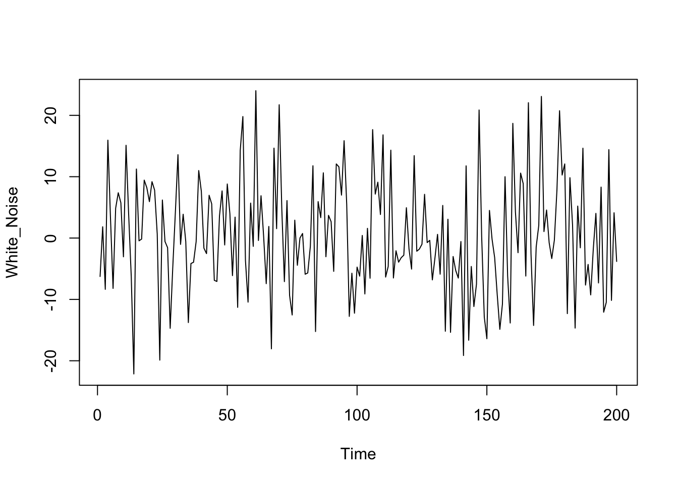
White noise processes are stationary.
The above plot of a simulated white noise process is typical of a stationary process. Evidence for stationarity, or more accurately evidence for non-stationarity, can be observed on a time plot of a given time series.
Prove Lemma 7.2.6
Consider the time series \(\{ X_t : t \in \mathbb{Z} \}\) defined by \[X_t = \frac{1}{2} X_{t-1} + Z_t\] where \(\{ Z_t \}\) is a white noise process with variance \(\sigma^2\). Is this time series stationary or non-stationary?
By iteratively applying the definition of the time series observe that
\[\begin{align*}
X_t &= \frac{1}{2} X_{t-1} + Z_t \\[3pt]
&= \frac{1}{2}\left( \frac{1}{2} X_{t-2} + Z_{t-1} \right) + Z_t \\[3pt]
&= \frac{1}{2^2} X_{t-2} + \frac{1}{2} Z_{t-1} + Z_t \\[3pt]
&= \frac{1}{2^2} \left( \frac{1}{2} X_{t-3} + Z_{t-2} \right) + \frac{1}{2} Z_{t-1} + Z_t \\[3pt]
&= \frac{1}{2^3} X_{t-3} + \frac{1}{2^2} Z_{t-2} + \frac{1}{2} Z_{t-1} + Z_t \\[3pt]
& \vdots \\[3pt]
&= \sum\limits_{j=0}^{\infty} \frac{1}{2^j} Z_{t-j}.
\end{align*}\]
This identity allows us to calculate \[\begin{align*} \mathbb{E}(X_t) &= \mathbb{E} \left( \sum\limits_{j=0}^{\infty} \frac{1}{2^j} Z_{t-j} \right) \\[3pt] &= \sum\limits_{j=0}^{\infty} \frac{1}{2^j} \mathbb{E} (Z_{t-j}) \\[3pt] &= \sum\limits_{j=0}^{\infty} \frac{1}{2^j} \cdot 0 \\[3pt] &= 0. \end{align*}\] So the random variables in the time series have the same expectation. Similarly \[\begin{align*} \text{Var} (X_t) &= \text{Var} \left( \sum\limits_{j=0}^{\infty} \frac{1}{2^j} Z_{t-j} \right) \\[3pt] &= \sum\limits_{j=0}^{\infty} \text{Var} \left( \frac{1}{2^j}Z_{t-j} \right) + \sum\limits_{i \neq j} \text{Cov} \left( \frac{1}{2^i}Z_{t-i},\frac{1}{2^j}Z_{t-j} \right) \\[3pt] &= \sum\limits_{j=0}^{\infty} \left( \frac{1}{2^j} \right)^2 \text{Var} \left( Z_{t-j} \right) + \sum\limits_{i \neq j} 0 \\[3pt] &= \sigma^2 \sum\limits_{j=0}^{\infty} \frac{1}{4^j} \\[3pt] &= \sigma^2 \left( \frac{1}{1-\frac{1}{4}} \right) \\[3pt] &= \frac{4}{3} \sigma^2. \end{align*}\] So the random variables in the time series have the same finite non-zero variation. Finally \[\begin{align*} \text{Cov} (X_t, X_{t+h}) &= \mathbb{E} \left[ X_t X_{t+h} \right] - \mathbb{E} \left[ X_t \right] \mathbb{E} \left[ X_{t+h} \right] \\[5pt] &= \mathbb{E} \left[ X_t X_{t+h} \right] \\[5pt] &= \mathbb{E} \left[ \left( \sum\limits_{j=0}^{\infty} \frac{1}{2^j} Z_{t-j} \right) \left( \sum\limits_{k=0}^{\infty} \frac{1}{2^k} Z_{t+h-k} \right) \right] \\[5pt] &= \sum\limits_{j=0}^{\infty} \sum\limits_{k=0}^{\infty} \frac{1}{2^j} \frac{1}{2^k} \mathbb{E} \left[ Z_{t-j} Z_{t+h-k} \right] \end{align*}\]
Now when \(t-j \neq t+h-k\), or equivalently \(k \neq j+h\), then \(\mathbb{E} \left[ Z_{t-j} Z_{t+h-k} \right] = \mathbb{E} \left[ Z_{t-j} \right] \mathbb{E} \left[ Z_{t+h-k} \right] = 0\) using independence of the random variables. It follows that \[\begin{align*} \text{Cov} (X_t, X_{t+h}) &= \sum\limits_{j=0}^{\infty} \sum\limits_{k=0}^{\infty} \frac{1}{2^j} \frac{1}{2^k} \mathbb{E} \left[ Z_{t-j} Z_{t+h-k} \right] \\[5pt] &= \sum\limits_{j=0}^{\infty} \frac{1}{2^j} \frac{1}{2^{j+h}} \mathbb{E} \left[ Z_{t-j}^2 \right] \\[3pt] &= \frac{\sigma^2}{2^h} \sum\limits_{j=0}^{\infty} \frac{1}{4^j} \\[3pt] &= \frac{\sigma^2}{2^h} \left( \frac{1}{1-\frac{1}{4}} \right) \\[3pt] &= \frac{4 \sigma^2}{3 \cdot 2^h}. \end{align*}\] So \(\text{Cov} (X_t, X_{t+h})\) depends only on \(h\), not on \(t\).
These three points together show that the time series is stationary.Consider the time series \(\{ X_t : t \in \mathbb{Z} \}\) defined by \[X_t = X_{t-1} + Z_t\] where \(\{ Z_t \}\) is a white noise process with variance \(\sigma^2\). Is this time series stationary or non-stationary?
By iteratively applying the definition of the time series observe that
\[\begin{align*}
X_t &= X_{t-1} + Z_t \\[3pt]
&= X_{t-2} + Z_{t-1} + Z_t \\[3pt]
&= X_{t-3} + Z_{t-2} + Z_{t-1} + Z_t \\[3pt]
& \vdots \\[3pt]
&= \sum\limits_{j=0}^{\infty} Z_{t-j}.
\end{align*}\]
The time series \(\{ X_t : t \in \mathbb{Z} \}\) in Example 7.2.8 is known as a random walk. Note that \(X_t - X_{t-1}\) is a stationary time series. This can be proved directly from the definition, or by exploiting the identity \(X_t - X_{t-1} = Z_{t}\) where \(Z_t\) is a white noise process which is known to be stationary. This illustrates a useful phenomenon where time series can be translated to a stationary time series.
Produce time plots in R for the time series in Example 7.2.7 and Example 7.2.8. Are these plots consistent with the solutions to the examples?
7.3 Moving Average, General Linear and Autoregressive Processes
In this section we introduce a number of examples of time series. These examples are highly flexible, and play an important role when it comes to fitting time series models and forecasting.
Let \(\{ Z_t : t \in \mathbb{Z} \}\) be a white noise process with variance \(\sigma^2\). Define a time series \(\{ X_t : t \in \mathbb{Z} \}\) by \[X_t = Z_t + \theta_1 Z_{t-1} + \ldots + \theta_q Z_{t-q},\] where \(\theta_1, \ldots, \theta_q\) are constants. This time series is known as a moving average process of order \(q\), and is often denoted \(MA(q)\).
Definition 7.3.1 specifies that \(X_t\) is a linear combination of present and past noise components.
Moving average processes can be simulated in R. The following code produces \(200\) samples from a moving average process \(MA(2)\) with parameters \(\theta_1=0.5, \theta_2 = 0.2\) and where the white noise processes has a standard deviation \(10\), or equivalently variance \(100\).
The time series \(MA(q)\) is stationary.
It is routine to check that \[\begin{align*} \mathbb{E} \left( X_t \right) &= \mathbb{E} \left( Z_t + \theta_1 Z_{t-1} + \ldots + \theta_q Z_{t-q} \right) \\[5pt] &= \mathbb{E} \left( Z_t \right) + \theta_1 \mathbb{E} \left( Z_{t-1} \right) + \ldots + \theta_q \mathbb{E} \left( Z_{t-q} \right) \\[5pt] &= 0 + \theta_1 \cdot 0 + \ldots + \theta_q \cdot 0 \\[5pt] &= 0, \end{align*}\] and \[\begin{align*} \text{Var} \left( X_t \right) &= \text{Var} \left( Z_t + \theta_1 Z_{t-1} + \ldots + \theta_q Z_{t-q} \right) \\[5pt] &= \sum\limits_{j=0}^{q} \text{Var} \left( \theta_j Z_{t-j} \right) + \sum\limits_{i,j=0 \\ i \neq j}^{q} \text{Cov}(\theta_i Z_{t-i},\theta_j Z_{t-j}) \\[5pt] &= \sum\limits_{j=0}^{q} \theta_j^2 \text{Var} \left(Z_{t-j} \right) + \sum\limits_{i,j=0 \\ i \neq j}^{q} 0 \\[5pt] &= \sigma^2 \sum\limits_{j=0}^{q} \theta_j^2. \\[5pt] \end{align*}\] where we have set \(\theta_0=1\). So \(\mathbb{E} \left( X_t \right)\) and \(\text{Var} \left( X_t \right)\) are independent of \(t\).
Now calculating the covariance of the random variables of the time series: \[\begin{align*} \text{Cov} \left( X_t, X_{t+h} \right) &= \mathbb{E} \left( X_t X_{t+h} \right) - \mathbb{E} \left( X_t \right) \mathbb{E} \left( X_{t+h} \right) \\[5pt] &= \mathbb{E} \left( X_t X_{t+h} \right) \\[5pt] &= \mathbb{E} \left[ \left( \sum\limits_{j=0}^q \theta_j Z_{t-j} \right) \left( \sum\limits_{k=0}^q \theta_k Z_{t+h-k} \right) \right] \\[5pt] &= \sum\limits_{j=0}^q \sum\limits_{k=0}^q \theta_j \theta_k \mathbb{E} \left( Z_{t-j} Z_{t+h-k} \right) \end{align*}\]
Since \(Z_{t-j}\) and \(Z_{t+h-j}\) are independent unless \(Z_{t-j}=Z_{t+h-k}\) which only occurs if \(k=j+h\). This does not occur in the expression \(\sum\limits_{j=0}^q \sum\limits_{k=0}^q \theta_j \theta_k \mathbb{E} \left( Z_{t-j} Z_{t+h-k} \right)\) if \(h>q\). Alternatively if \(0 \leq h \leq q\), then the expression reduces to become \(\sigma^2 \sum\limits_{j=0}^{q-h} \theta_j \theta_{j+h}\). It follows that \[\begin{align*} \text{Cov} \left( X_t, X_{t+h} \right) &= \sum\limits_{j=0}^q \sum\limits_{k=0}^q \theta_j \theta_k \mathbb{E} \left( Z_{t-j} Z_{t+h-k} \right) \\[9pt] &= \begin{cases} 0, & \text{ if } h >q \\[3pt] \sigma^2 \sum\limits_{j=0}^{q-h} \theta_j \theta_{j+h}, & \text{ if } 0 \leq h \leq q \end{cases} \end{align*}\] Therefore \(\text{Cov} \left( X_t, X_{t+h} \right)\) depends only on \(h\), not on \(t\).
It follows that \(MA(q)\) a stationary time series.
We see that a feature of the \(MA(q)\) is that the covariance, and therefore the correlation, between random variables cuts off after a lag of \(q\).
Let \(\{ Z_t : t \in \mathbb{Z} \}\) be a white noise process with variance \(\sigma^2\). Define a time series \(\{ X_t : t \in \mathbb{Z} \}\) by \[X_t = \sum\limits_{j=0}^{\infty} \alpha_j Z_{t-j},\] where \(\alpha_j\) are constants. This time series is known as a general linear process.
Note that the defintion of a general linear process is similar to a moving average process of infinite order. For this reason general linear processes are often denoted by \(MA(\infty)\).
It can be shown, in a very similar fashion to the proof of Lemma 7.3.2, that for a general linear process \(\{ X_t : t \in \mathbb{Z} \}\) we have
\(\mathbb{E}(X_t) =0\);
\(\text{Var}(X_t) = \sigma^2 \sum\limits_{j=0}^{\infty} \alpha_j^2\);
\(\text{Cov} (X_t,X_{t+h}) = \sigma^2 \sum\limits_{j=0}^{\infty} \alpha_j \alpha_{j+h}\).
This leads to the following statement.
A general linear process time series \(MA( \infty )\) is stationary if and only if \(\sum\limits_{j=0}^{\infty} \alpha_j^2 < \infty\).
Let \(\{ Z_t : t \in \mathbb{Z} \}\) be a white noise process with variance \(\sigma^2\). Define a time series \(\{ X_t : t \in \mathbb{Z} \}\) by \[X_t = \phi_1 X_{t-1} + \phi_2 X_{t-2} + \ldots + \phi_{p} X_{t-p} + Z_t,\] where \(\phi_j\) are constants. This time series is known as an autoregressive process of order \(p\), and is often denoted \(AR(p)\).
Definition 7.3.5 specifies that \(X_t\) is a linear combination of past time series observations and a white noise error term.
Autoregressive processes can be simulated in R. The following code produces \(200\) samples from an autoregressive process \(AR(2)\) with parameters \(\phi_1=0.5, \phi_2 = 0.2\) and where the white noise processes has a standard deviation \(10\), or equivalently variance \(100\).
Note that the arima.sim function only works if the simulated time series is stationary. Proving stationarity for \(AR(p)\) is significantly more difficult. We omit the proofs of the following two lemmas.
An \(AR(p)\) process is stationary if and only if the roots of the equation \[1 - \phi_1 x - \phi_2 x^2 - \ldots - \phi_p x^p=0,\] have absolute value strictly greater than \(1\).
Consider the \(AR(2)\) process \(\{ X_t : t \in \mathbb{Z} \}\) where \[X_t = \frac{3}{4} X_{t-1}- \frac{1}{8}X_{t-2} + Z_t\] Is this time series stationary?
In the notation of Definition 7.3.5, we have \(\phi_1 = \frac{3}{4}\) and \(\phi_2 = -\frac{1}{8}\). Following Lemma 7.3.6, consider the equation: \[\begin{align*} 1 - \frac{3}{4} x + \frac{1}{8} x^2 &= 0 \\[3pt] x^2 -6x+8 &= 0 \\[3pt] (x-2)(x-4) &= 0 \end{align*}\] The equation has roots \(2\) and \(4\). Clearly \(\lvert 2 \rvert, \lvert 4 \rvert > 1\), so by Lemma 7.3.6, the time series is stationary.
The expectations, variances and correlation of the random variables in a stationary \(AR(p)\) process are given by \[\begin{align*} \mathbb{E}(X_t) &= 0, \\[9pt] \text{Var}(X_t) &= \sigma^2 \sum\limits_{j=0}^{\infty} \beta_j^2, \\[9pt] \rho(X_t, X_{t+h}) &= \frac{\sum\limits_{j=0}^{\infty} \beta_j \beta_{j+h}}{\sum\limits_{j=0}^{\infty} \beta_j^2}, \end{align*}\] where \[\frac{1}{1 - \phi_1 x - \phi_2 x^2 - \ldots - \phi_p x^p} = 1 + \beta_1 x + \beta_2 x^2 + \ldots\]
Calculating the values \(\beta_j\) is often difficult in practice.
Consider the \(AR(1)\) process \(\{ X_t : t \in \mathbb{Z} \}\) where \[X_t = \frac{1}{2} X_{t-1} + Z_t.\] Calculate the expectation, the variance and the correlation of the random variables from the time series.
In the notation of Definition 7.3.5, we have \(\phi_1 = \frac{1}{2}.\)
By Taylor’s theorem applied to \(\frac{1}{1-\frac{1}{2}x}\) we have
\[\frac{1}{1-\frac{1}{2}x} = 1 + \frac{1}{2} x + \frac{1}{4} x^2 + \frac{1}{8} x^3 + \ldots,\]
and so in the notation of Lemma 7.3.8, we have \(\beta_j = \left( \frac{1}{2} \right)^j\). The lemma then tells us that
\[\begin{align*}
\mathbb{E}(X_t) &= 0 \\[5pt]
\text{Var}(X_t) &= \sigma^2 \sum\limits_{j=0}^{\infty} \left( \frac{1}{2^j} \right)^2 \\[5pt]
&= \sigma^2 \sum\limits_{j=0}^{\infty} \frac{1}{4^j} \\[5pt]
&= \sigma^2 \left( \frac{1}{1-\frac{1}{4}} \right) \\[5pt]
&= \frac{4}{3} \sigma^2 \\[5pt]
\rho (X_t,X_{t+h}) &= \frac{\sum\limits_{j=0}^{\infty} \left( \frac{1}{2} \right)^j \left( \frac{1}{2} \right)^{j+h}}{\sum\limits_{j=0}^{\infty} \left( \frac{1}{2} \right)^{2j}} \\[5pt]
&= \left( \frac{1}{2} \right)^{h} \left( \frac{\sum\limits_{j=0}^{\infty} \left( \frac{1}{2} \right)^{2j}}{\sum\limits_{j=0}^{\infty} \left( \frac{1}{2} \right)^{2j}} \right) \\[5pt]
&= \frac{1}{2^h}
\end{align*}\]
In general, autoregressive processes indicate previous observations have a direct effect on the time series and moving average processes indicate the previous errors have more of an impact. This is a key point when it comes to deciding on a time series model that you might want to fit to your own data.
As further reading for the module, you may wish to study autoregressive moving average processes, denoted \(ARMA(p,q)\). These models indicate both previous observations and previous errors have an impact on the time series.
7.4 Fitting
So far much of the discussion has been theoretical discussing stationarity as well as the measures of expectation, variance covariance and correlation in the context of time series.
However as professional industry data scientists, we are interested in applying the theory to the workplace. Suppose one has observed some time series data \(x_1, x_2, \ldots, x_n\). How does one fit a model time series to the realised data? It is important we can do this so that we ultimately can make inferences and predictions about our time series.
As a first step we have already seen that evidence for stationarity can best be observed in a time plot. Most of the theoretical models we have seen so far are stationary, and so in order to fit a model to our data, we need our data to reasonably come from a stationary distribution. So what if our data exhibits trend or seasonality: features known to break stationarity?
To remove seasonality from a time series dataset \(\{ X_t : t \in \mathbb{Z} \}\), then one should identify the length \(d\) of the cycles and instead of fitting a model to \(\{ X_t : t \in \mathbb{Z} \}\), one should fit a model to the translated time series data \(\{ W_t = X_t - X_{t-d} : t\in \mathbb{Z}\}\).
To remove trend from a time series dataset \(\{ X_t : t \in \mathbb{Z} \}\), then one should estimate the general trend by a polynomial of degree \(d\). and instead of fitting a model to \(\{ X_t : t \in \mathbb{Z} \}\), one should fit a model to the translated time series data \(\{ W_t: t\in \mathbb{Z}\}\) where \[W_t = X_t -{d \choose 1} X_{t-1} + {d \choose 2} X_{t-2} - \ldots + (-1)^{d-1} {d \choose d-1} X_{t-d+1} + (-1)^d X_{t-d}.\]
Supposing stationarity seems like a reasonable assumption from the time plot, then the theoretical measures can be estimated by sample statistics. In particular, the random variables have a common mean, and this can be estimated by \[\bar{x} = \frac{1}{n} \sum\limits_{t=1}^{n} x_i.\] Similarly the random variables have a common variance, and this can be estimated by \[c_0 = \frac{1}{n} \sum\limits_{t=1}^n \left( x_t- \bar{x} \right)^2.\] The covariance between \(X_t\) and \(X_{t+h}\) is estimated by \[c_h = \frac{1}{n} \sum\limits_{t=1}^{n-h} (x_t - \bar{x})(x_{t+h}-\bar{x}),\] meaning the sample correlation is \[r_h = \frac{\sum\limits_{t=1}^{n-h} (x_t - \bar{x})(x_{t+h}-\bar{x})}{\sum\limits_{t=1}^n \left( x_t- \bar{x} \right)^2}.\]
In particular, calculating the sample correlations is a key step in time series model selection. Typically one should calculate sample correlations \(r_1, r_2, \ldots, r_{30}\). These can then by plotted in a correlogram: a plot of \(r_h\) against \(h\).
Given time series data the acf function can be used to plot the correlogram. The following code plot the correlogram for the dfw.2011 time series data in the tswge package.
By comparing this correlogram against a similar plot of the theoretical correlations against time for proposed time series models, one can identify sensible model choices.
The following code plots the theoretical correlogram for the \(MA(2)\) process with parameters \(\theta_0 = 0.5, \theta_1 = 0.2\).
theory_cors=ARMAacf(ma=c(0.5,0.2), lag.max=30)
plot(theory_cors,
     main="",
     xlab="h",
     ylab="Theoretical Correlation",
     type="b")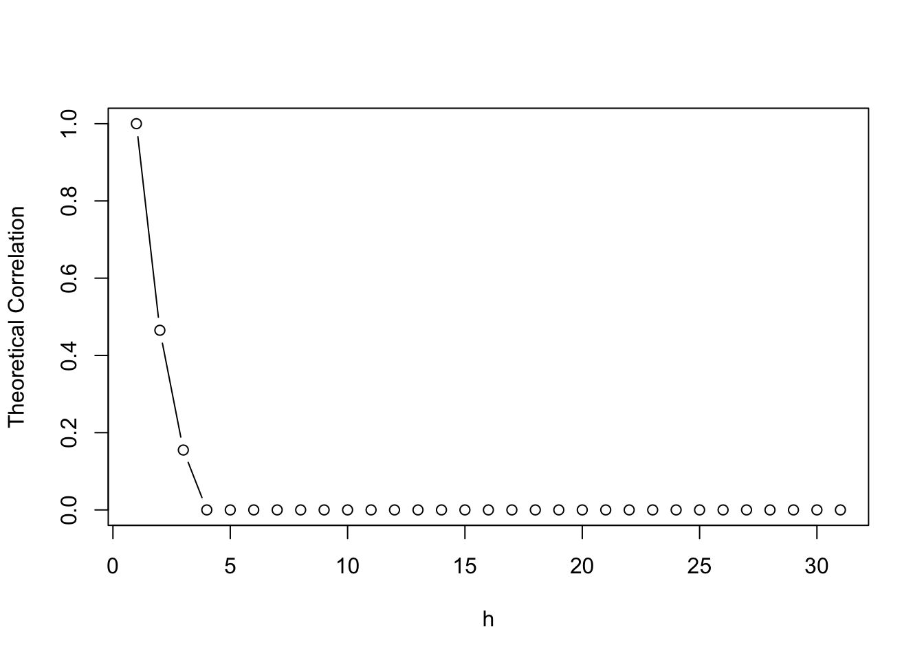
An \(MA(q)\) process will have a theoretical correlation that drops sharply to \(0\) for values of \(h\) larger than \(q\). This is consistant with the workings of Lemma 7.3.2.
The following code plots the theoretical correlogram for the \(AR(2)\) process with parameters \(\phi_1 = 0.5, \phi_2 = 0.2\).
theory_cors=ARMAacf(ar=c(0.5,0.2), lag.max=30)
plot(theory_cors,
     main="",
     xlab="h",
     ylab="Theoretical Correlation",
     type="b")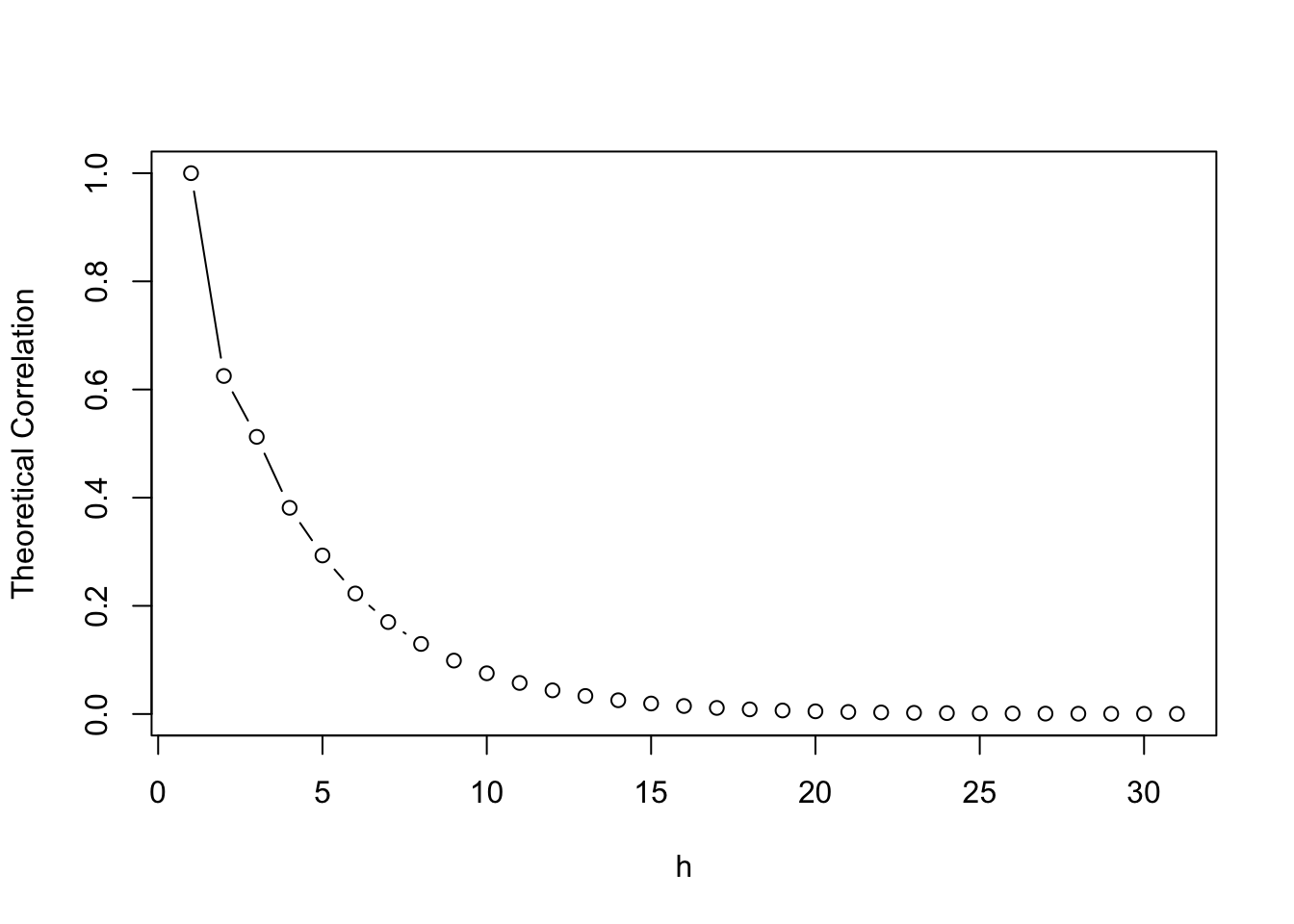
Typically a stationary \(AP(p)\) process will have a theoretical correlation that decays exponentially with \(h\). A quicker decay indicates smaller \(p\).
As further reading for the module, you may wish to study partial correlations. Informally the partial correlation between \(X_t\) and \(X_{t+h}\) is a measure of the correlation between \(X_t\) and \(X_{t+h}\) with the effect of \(X_{t+1},X_{t+2}, \ldots, X_{t+h-1}\) removed. As with correlation leading to correlograms, partial correlations lead to partial correlograms. These partial correlograms of observed data (plotted with pacf in R) can be compared with theoretical partial correlograms for additional insight towards suitable model choices.
Consider the following sequential time series data: \[1.70361316, \quad 1.39819724, \quad 3.65999528, \quad 3.25475575, \quad 3.61901954, \quad 3.28511974,\] \[2.21333456, \quad 2.18079340, \quad 0.15775543, \quad 1.60753475, \quad 1.60003461, \quad 3.61264282,\] \[3.72688807, \quad 2.64425283, \quad 2.99055390, \quad 1.75740088, \quad 0.32802739, \quad 0.58667089,\] \[0.08471193, \quad 0.07734609, \quad 0.14395280, \quad -0.45996343, \quad -0.98263582, \quad -1.01955085,\] \[0.26049123, \quad -1.28912469, \quad -0.56626603, \quad -0.17668906, \quad 0.90407968, \quad 0.50948779.\] What would be a sensible choice of model?
First we write code to create a time plot of the data:
data = c(1.70361316,  1.39819724,  3.65999528,  3.25475575, 3.61901954,  3.28511974,
         2.21333456,  2.18079340,  0.15775543,  1.60753475,  1.60003461,  3.61264282,
         3.72688807,  2.64425283,  2.99055390,  1.75740088,  0.32802739,  0.58667089,
         0.08471193,  0.07734609,  0.14395280, -0.45996343, -0.98263582, -1.01955085,
         0.26049123, -1.28912469, -0.56626603, -0.17668906,  0.90407968,  0.50948779)
data = ts(data)
plot.ts(data)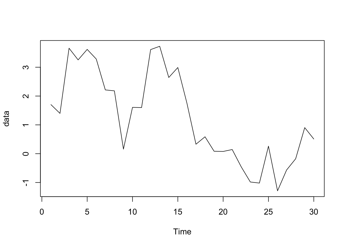
There is little to suggest that the data is not stationary. Therefore we are free to study the correlogram of the data:
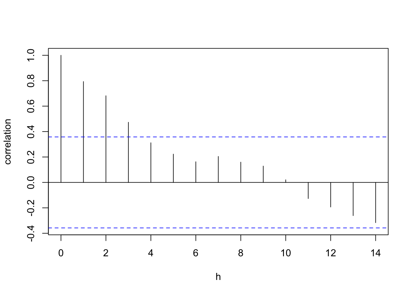
The blue dashed horizontal lines in this plot here mark \(y= \pm \frac{2}{\sqrt{n}}\). The data has very quickly decayed exponentially into this range suggesting that an \(AR(p)\) time series model with a small value of \(p\) would a sensible fit for our data.
Perform some further analysis of the data in Example 7.4.1. In particular study the partial correlogram of the data and compare with the partial correlogram of \(AR(p)\) for small \(p\). Is there a particular value of \(p\) this may suggest?
Consider the following sequential time series data: \[-0.12958358, \quad -0.74380695, \quad 1.17746650, \quad 1.12714817, \quad -0.65571450, \quad 0.07719486,\] \[0.98203923, \quad 0.94494370, \quad -0.01749771, \quad 1.35908697, \quad 1.14573382, \quad -0.42631896,\] \[-2.52532018, \quad 0.01758097, \quad 0.51753185, \quad -0.03865707, \quad 0.93574108, \quad 1.29313930,\] \[1.00451192, \quad 1.21592803, \quad 1.24162499, \quad 0.46563313, \quad -1.95206920, \quad -0.37485010,\] \[0.25378413, \quad -0.18385988, \quad -1.54865014, \quad -1.21352625, \quad 0.17886653, \quad 1.56765033.\] What would be a sensible choice of model?
First we write code to create a time plot of the data:
data = c(-0.12958358, -0.74380695, 1.17746650, 1.12714817, -0.65571450, 0.07719486,
         0.98203923, 0.94494370, -0.01749771, 1.35908697, 1.14573382, -0.42631896,
         -2.52532018, 0.01758097, 0.51753185, -0.03865707, 0.93574108, 1.29313930,
         1.00451192, 1.21592803, 1.24162499, 0.46563313, -1.95206920, -0.37485010,
         0.25378413, -0.18385988, -1.54865014, -1.21352625, 0.17886653, 1.56765033)
data = ts(data)
plot.ts(data)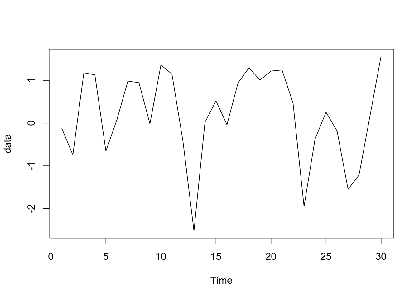
There is little to suggest that the data is not stationary. Therefore we are free to study the correlogram of the data:

Once a suitable choice of time series model has been made for the data, such as is the case in Example 7.4.1 and Example 7.4.2, it remains to estimate the parameters involved in the model. For example, an \(AR(1)\) model requires an estimation of the coefficient \(\phi_1\), and an \(MA(1)\) model requires an estimation of the coefficient \(\theta_1\).
The preferred technique to do this by is using the technique of maximum likelihood estimators, applied to \(X_t - \bar{x}\). For computational reasons, it is almost always best to do this using R, or another programming language, as opposed to direct calculation. R has a built-in functions arima to estimate parameters in this fashion. Code to fit both moving average processes and autoregression processes is illustrated in the following examples.
Consider again the data from Example 7.4.1. Estimate the parameters to fit a \(AR(1)\) process to the data.
To do this we run the following code:
data = c(1.70361316,  1.39819724,  3.65999528,  3.25475575, 3.61901954,  3.28511974,
         2.21333456,  2.18079340,  0.15775543,  1.60753475,  1.60003461,  3.61264282,
         3.72688807,  2.64425283,  2.99055390,  1.75740088,  0.32802739,  0.58667089,
         0.08471193,  0.07734609,  0.14395280, -0.45996343, -0.98263582, -1.01955085,
         0.26049123, -1.28912469, -0.56626603, -0.17668906,  0.90407968,  0.50948779)
data = ts(data)
model <-arima(data,order=c(1,0,0),method="ML")
model
This returns
##
## Call:
## arima(x = data, order = c(1, 0, 0), method = "ML")
##
## Coefficients:
##          ar1  intercept
##       0.7777     1.2313
## s.e.  0.1045     0.6905
##
## sigma^2 estimated as 0.8712: log likelihood = -40.96, aic = 87.93Note in the example that the standard error of the estimations is also presented.
Consider again the data from Example 7.4.2. Estimate the parameters to fit a \(MA(1)\) process to the data.
To do this we run the following code:
data = c(-0.12958358, -0.74380695, 1.17746650, 1.12714817, -0.65571450, 0.07719486,
         0.98203923, 0.94494370, -0.01749771, 1.35908697, 1.14573382, -0.42631896,
         -2.52532018, 0.01758097, 0.51753185, -0.03865707, 0.93574108, 1.29313930,
         1.00451192, 1.21592803, 1.24162499, 0.46563313, -1.95206920, -0.37485010,
         0.25378413, -0.18385988, -1.54865014, -1.21352625, 0.17886653, 1.56765033)
data = ts(data)
model <-arima(data,order=c(0,0,1),method="ML")
model
This returns
##
## Call:
## arima(x = data, order = c(0, 0, 1), method = "ML")
##
## Coefficients:
##          ma1  intercept
##       0.5254     0.2152
## s.e.  0.1405     0.2529
##
## sigma^2 estimated as 0.8424: log likelihood = -40.16, aic = 86.31In summary, fitting typically follows the following steps:
Produce a time plot of observed data \(x_1, x_2, \ldots, x_n\)? Does the data look stationary? If not, translate data to remove seasonality, trend and changing variance as appropriate;
Calculate sample correlations of \(X_t\) and \(X_{t+h}\). Produce a correlogram, and compare to theoretical forms for different time series models. If deemed necessary repeat for partial correlations;
Identify appropriate time series model;
Estimate parameters to fit a model to \(X_t - \bar{x}\).
Once we have fitted our model, we are able to use this to make predicts for future observations (of the translated data).
7.5 Forecasting
An important aspect of time series analysis is predicting the behavior of a time series in the future. This is known as forecasting.
Broadly speaking to perform forcasting given the time series observations \(x_1, x_2, \ldots, x_n\), one should fit a model as per the steps at the end of Section 7.4, and then use the model to make predictions for the times series. Note the predictions may subsequently need translated back to the scale of the original data (prior to translation to guarentee stationarity).
In general we denote a prediction for \(X_t\) by \(\hat{x}_t\).
For \(AR(2)\) processes and the more general \(AR(p)\) processes, the following theorems tell us how to make predictions.
Suppose we have some time series data \(x_1,x_2,\ldots ,x_n\) to which we have fitted the \(AR(2)\) model \[X_t = \phi_1 X_{t-1} + \phi_2 X_{t-2} + Z_t.\] Then the model predicts that \(X_{n+k}\) is given by \[\hat{x}_{n+k} = \frac{\lambda_1^{k+1} - \lambda_2^{k+1}}{\lambda_1 - \lambda_2} X_n - \frac{\lambda_2 \lambda_1^{k+1} - \lambda_1 \lambda_2^{k+1}}{\lambda_1 - \lambda_2} X_{n-1},\] where \(\frac{1}{\lambda_1}, \frac{1}{\lambda_2}\) are the roots of the equation \(1 - \phi_1 x - \phi_2 x^2 = 0\).
Consider the \(AR(2)\) process \(\{ X_t : t \in \mathbb{Z} \}\) where \[X_t = \frac{3}{4} X_{t-1}- \frac{1}{8}X_{t-2} + Z_t.\] If observations \(x_1, x_2, \ldots, x_n\) are made, what are the predicted values \(\hat{x}_{n+1}\) and \(\hat{x}_{n+2}\).
Recall from Example 7.3.7, that the roots of \(1 - \frac{3}{4} x - \frac{1}{8} x^2 =0\) are \(2\) and \(4\). Therefore \(\lambda_1 = \frac{1}{2}\) and \(\lambda_2 = \frac{1}{4}\). It follows from taking \(k=1\) and \(k=2\) in Theorem 7.5.1 that \[\begin{align*} \hat{x}_{n+1} &= \frac{\left( \frac{1}{2} \right)^2 - \left( \frac{1}{4} \right)^2}{\frac{1}{2} -\frac{1}{4}} x_n - \frac{\frac{1}{4} \left( \frac{1}{2} \right)^2 - \frac{1}{2}\left( \frac{1}{4} \right)^2}{\frac{1}{2} - \frac{1}{4}} x_{n-1} \\[9pt] &= \frac{\frac{1}{4} - \frac{1}{16}}{\frac{1}{4}} x_n - \frac{\frac{1}{16} - \frac{1}{32}}{\frac{1}{4}} x_{n-1} \\[9pt] &= \frac{3}{4} x_n - \frac{1}{8} x_{n-1} \\[9pt] \hat{x}_{n+2} &= \frac{\left( \frac{1}{2} \right)^3 - \left( \frac{1}{4} \right)^3}{\frac{1}{2} -\frac{1}{4}} x_n - \frac{\frac{1}{4} \left( \frac{1}{2} \right)^3 - \frac{1}{2}\left( \frac{1}{4} \right)^3}{\frac{1}{2} - \frac{1}{4}} x_{n-1} \\[9pt] &= \frac{\frac{1}{8} - \frac{1}{64}}{\frac{1}{4}} x_n - \frac{\frac{1}{32} - \frac{1}{128}}{\frac{1}{4}} x_{n-1} \\[9pt] &= \frac{7}{16} x_n - \frac{3}{32} x_{n-1}. \end{align*}\]
Suppose we have some time series data \(x_1,x_2,\ldots ,x_n\) to which we have fitted the \(AR(p)\) model \[X_t = \phi_1 X_{t-1} + \phi_2 X_{t-2} + \cdots + \phi_p X_{t-p} + Z_t.\] Then the model predicts that \(X_{n+k}\) is given by \[\hat{x}_{n+k} = \phi_1 \hat{x}_{n+k-1} + \phi_2 \hat{x}_{n+k-2} + \ldots + \phi_p \hat{x}_{n+k-p},\] where \(\hat{x}_{j}\) is replaced by \(x_j\) if \(j \leq n\).
Of course, if your time series is fitted by an alternative time series model, such as an \(MA(P)\) model or an \(ARMA(p,q)\) model, then these theorems may not be of use to you. Some further reading may be required. As a data scientist it is important to have the skill of being able to broaden your knowledge independently when required by your data!
The forecast function can be used in R to make future predictions using fitted models from Section 7.4. Within this function the level parameter can be used to give bounds for confidence intervals. This is illustrated in the following example.
Consider again the data from Example 7.4.2. Make predictions for the next \(6\) time steps.
Inspired by the fitted model of Example 7.4.3, run the code:
library(forecast)
data = c(1.70361316,  1.39819724,  3.65999528,  3.25475575, 3.61901954,  3.28511974,
         2.21333456,  2.18079340,  0.15775543,  1.60753475,  1.60003461,  3.61264282,
         3.72688807,  2.64425283,  2.99055390,  1.75740088,  0.32802739,  0.58667089,
         0.08471193,  0.07734609,  0.14395280, -0.45996343, -0.98263582, -1.01955085,
         0.26049123, -1.28912469, -0.56626603, -0.17668906,  0.90407968,  0.50948779)
data = ts(data)
mod <-arima(data,order=c(1,0,0),method="ML")
pred <- forecast(data,h=6,model=mod,level=95)
predThere a number of sources of error in forecasting that one should be aware of:
An incorrect model may have been fitted. This could come from a poor choice of standard time series to fit, or from poor choice of parameters within a correct choice of standard time series.
Even if a model fits data well, there will inevitably be uncertainty in each parameter estimation. This uncertainty can and should be accounted for when making and communicating predictions.
Making a prediction for \(X_{n+k}\) having observed data up to time \(t=n\) usually involves future values of white noise \(Z_{n+1}, \ldots, Z_{n+k}\). However these are unknown and therefore introduce another source of uncertainty. Our uncertainty bounds will increase the further into the future we wish to make predictions.