Chapter 10 Equilibrium Distributions
Consider the Markov Chain governing Mary Berrys’ choice of Nottingham coffee shop of Example 8.1.3, that is the Markov chain described by the diagram

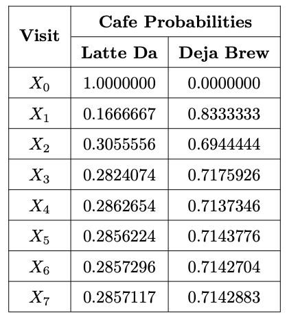
Suppose that Mary Berry visits Latte Da on her first trip to Nottingham, that is \(X_0= \text{Latte Da}\). The probabilities that Mary Berry visits either coffee shop on her \(n^{th}\) visit to Nottingham are displayed in the following table:
This calculation can be verified using the following R code:
x <- matrix(c(1/6,5/6,1/3,2/3),nrow=2,byrow=T)
y <- matrix(c(1,0),nrow=1,byrow=T)
for (i in 1:25)
  y<- y %*% x
y
Alternatively suppose that Mary Berry visits Deja Brew on her first trip to Nottingham. This change in initial state means the probabilities that Mary Berry visits either coffee shop on her \(n^{th}\) visit to Nottingham are now as in the following table:
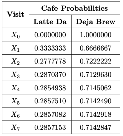
Note that the initial state \(X_0\) doesn’t appear to affect the long-term behavior of the Markov chain: the probability that Mary Berry goes to Latte Da on a suitably distant visit to Nottingham is approximately \(0.28571\) or \(\frac{2}{7}\) irrespective of which coffee shop she tries first. Equivalently the probability that Mary Berry goes to Deja Brew on a suitably distant visit to Nottingham is approximately \(0.71428\) or \(\frac{5}{7}\) irrespective of which coffee shop she tries firs. Mathematically one could say that the limiting behavior of the Markov chain seems to have distribution \(\left( \frac{2}{7}, \frac{5}{7} \right)\).
This type of long-term or limiting behaviour of Markov chains will be the focus of this chapter.
10.1 Definition of Equilibrium Distributions
Throughout this chapter consider a Markov chain with state space \(S\) and transition matrix \(P\).
Let \(e_i = (0,0,\ldots,0,1,0,\ldots,0)\) be the row vector where the \(1\) is in the \(i^{th}\) position. Then performing the matrix multiplication \(e_i \cdot P\) results in the vector \(( p_{i1}, p_{i2}, \ldots , p_{i \lvert S \rvert})\), that is the vector with the entry in the \(j^{th}\) position is the probability of moving to state \(j\) from \(i\).
More generally calculating \(e_i \cdot P^n\) gives the vector \(\left( p_{i1}^{(n)}, p_{i2}^{(n)}, \ldots , p_{i \lvert S \rvert}^{(n)} \right)\) that is the vector with the entry in the \(j^th\) position as the probability of moving to state \(j\) in \(n\) steps from state \(i\).
However this can generalise further: think of a row vector, which we seek to multiply on the left by \(P\), as describing the probability mass function of \(X_0\). So a row vector \(v = \left( v_1, v_2, \ldots, v_{\lvert S \rvert} \right)\) would be defined by \(v_i = P(X_0 = i)\). In this content, \(e_i\) would represent \(X_0\) being equal to \(i\) as a certain event, all other states for \(X_0\) are impossible. It then follows that \(v \cdot P\) describes the probability mass function of \(X_1\). More generally \(v \cdot P^n\) describes the probability mass function of \(X_n\).
Convince yourself, by direct calculation using \(v = \left( v_1, v_2, \ldots, v_{\lvert S \rvert} \right)\) and \(P = \left( p_{ij} \right)\), that \(v \cdot P\) gives the row vector whose \(j^{th}\) entry is \(P(X_1 =j)\).
The above discussion is crucial to the interpretation of the following definition:
A row vector \(\pi =(\pi_1, \pi_2, \ldots, \pi_{\lvert S \rvert})\) is called an equilibrium or stationary distribution of the Markov chain if
1.) \(\pi_i \geq 0\) for all states \(i\) in \(S\);
2.) \(\sum\limits_{i \in S} \pi_i = 1\);
3.) \(\pi P = \pi.\)
The first two conditions of Definition 10.1.1 are consequences of \(\pi_i\) representing a probability that the Markov chain is in state \(i\). The third condition of Definition 10.1.1 describes the Markov chain reaching a steady state.
Let \(\pi\) be an equilibrium distribution for some Markov chain and consider the quantities \(\pi P^2\) and \(\pi P^3\) respectively. Applying the identity \(\pi P = \pi\) from Definition 10.1.1, calculate: \[\begin{align*} \pi P^2 &= \left( \pi P \right) P = \left( \pi \right) P = \pi \\ \pi P^3 &= \left( \pi P\right) P^2 = \left( \pi \right) P^2 = \left( \pi P \right) P = \left(\pi \right) P = \pi. \end{align*}\] More generally, we can deduce that \[\pi P^n = \pi\] for any positive integer \(n\). This is to say that if \(P(X_0 = i) = \pi_i\) for all states \(i\), then \(P(X_n = i) = \pi_i\) for all positive integers \(n\).
10.2 Calculating Equilibrium Disrtributions
It often possible to calculate equilibrium distributions for Markov chains by using the transition matrix to deduce \(\lvert S \rvert\) equations for \(pi_1, pi_2, \ldots, pi_{\lvert S \rvert}\), that can be solved simultaneously alongside the ever present equation \(\sum\limits_{i \in S} \pi_i\) from Definition 10.1.1. R can be used to solve these simulataneously equations. This is all illustrated by the following example.
Find the equilibrium distribution of the Markov Chain governing Mary Berrys’ choice of Nottingham coffee shop of Example 8.1.3.
The transition matrix of the Markov chain is given by
\[\begin{pmatrix} \frac{1}{6} & \frac{5}{6} \\ \frac{1}{3} & \frac{2}{3} \end{pmatrix}\]
Therefore the equilibrium distribution will satisfy
\[\begin{align*}
& \qquad \begin{pmatrix} \pi_1 & \pi_2 \end{pmatrix} \begin{pmatrix} \frac{1}{6} & \frac{5}{6} \\ \frac{1}{3} & \frac{2}{3} \end{pmatrix} = \begin{pmatrix} \pi_1 & \pi_2 \end{pmatrix} \\[9pt]
\iff& \qquad \begin{pmatrix} \frac{1}{6} \pi_1 + \frac{1}{3} \pi_2 & \frac{5}{6} \pi_1 + \frac{2}{3} \pi_2 \end{pmatrix} = \begin{pmatrix} \pi_1 & \pi_2 \end{pmatrix} \\[9pt]
\iff& \qquad \begin{cases} \frac{1}{6} \pi_1 + \frac{1}{3} \pi_2 &= \pi_1 \\[3pt] \frac{5}{6} \pi_1 + \frac{2}{3} \pi_2 &= \pi_2 \end{cases} \\[9pt]
\iff& \qquad \begin{cases} -\frac{5}{6} \pi_1 + \frac{1}{3} \pi_2 &= 0 \\[3pt] \frac{5}{6} \pi_1 - \frac{1}{3} \pi_2 &= 0 \end{cases} \\[9pt]
\iff& \qquad \frac{5}{6} \pi_1 = \frac{1}{3} \pi_2.
\end{align*}\]
using the following R code:
We obtain \(\pi_1 = \frac{2}{7}\) and \(\pi_2 = \frac{5}{7}\). The equilibrium distribution of the Markov is \(\left( \frac{2}{7}, \frac{5}{7} \right)\).It is possible that the system of linear equations mentioned above does not solve to give a unique solution for \(\pi\). Indeed it is possible that there is no solution at all. We would like to understand when the equilibrium distribution exists, and if it does exist when it is unique. This is tackled by the following theorem.
An irreducible Markov chain has a unique equilibrium distribution \(\pi\) if and only if it is positive recurrent.
As well as solving the linear system above, there is another common identity that can used to find the equilibrium distribution supposing we know the mean recurrence times of each state, and vice-versa.
An irreducible Markov chain with a unique equilibrium distribution \(\pi\) satisfies \[\pi_i = \mu_i^{-1}, \qquad \text{for all states } i\] where \(\mu_i\) is the mean recurrence time of state \(i\).
In practice it is usually easier to calculate the equilibrium distribution of an irreducible Markov chain, than it is to calculate the mean recurrance times of every state.
Considering again the Markov chain of Example 8.1.3, calculate how many long in average (in terms of trips to Nottingham) the owners of Latte Da and Deja Brew will have to wait to see Mary Berry again.
Mathematically the question is asking us to calculate the mean recurrence times \(\mu_{\text{Latte Da}}\) and \(\mu_{\text{Deja Brew}}\) of Latte Da and Deja Brew respectively.
Sacred Heart Hospital have a fleet of ambulances across Greater Sacramento. The hospital owns four garages. At the beginning of each day every ambulance leaves its garage, completes nearby jobs transferring patients, and at the end of the day the ambulance parks in the garage nearest to its location. This may or may not be the same garage that the ambulance started the day in.
Based on data gathered through long term observation of the ambulances, the daily movement between garages is modelled by a Markov chain described by

Dr. Cox regularly leaves his stethoscope in the garage. How many working days will he expect to wait before he can pick it up again.
Mathematically, we are being asked to calculate the mean recurrence time of each state. To do this, we will prove the existence of and subsequently find a unique equilibrium distribution before appling Theorem 10.2.3 to obtain the mean recurrence times.
Note that clearly all states of the Markov chain are intercommunicating, that is, the Markov chain is irreducible. Furthermore since the Markov chain has only 4 states, by Lemma 9.3.9 the Markov chain is positive recurrent. Therefore by Theorem 10.2.2, there is a unique equalibrium distribution.
The probability transition matrix of the Markov chain is given by \[\begin{pmatrix} \frac{1}{2} & \frac{1}{4} & \frac{1}{4} & 0 \\ \frac{1}{6} & \frac{2}{3} & 0 & \frac{1}{6} \\ \frac{1}{4} & \frac{1}{4} & \frac{1}{4} & \frac{1}{4} \\ 0 & \frac{1}{6} & \frac{1}{3} & \frac{1}{2} \end{pmatrix}.\] The unique equalibrium distribution is the vector \(\pi =(\pi_1, \pi_2, \pi_3, \pi_4)\) satisfying \[\begin{align*} & \qquad \begin{pmatrix} \pi_1 & \pi_2 & \pi_3 & \pi_4 \end{pmatrix} \begin{pmatrix} \frac{1}{2} & \frac{1}{4} & \frac{1}{4} & 0 \\ \frac{1}{6} & \frac{2}{3} & 0 & \frac{1}{6} \\ \frac{1}{4} & \frac{1}{4} & \frac{1}{4} & \frac{1}{4} \\ 0 & \frac{1}{6} & \frac{1}{3} & \frac{1}{2} \end{pmatrix} = \begin{pmatrix} \pi_1 & \pi_2 & \pi_3 & \pi_4 \end{pmatrix} \\[9pt] \iff& \qquad \begin{pmatrix} \frac{1}{2} \pi_1 + \frac{1}{6} \pi_2 + \frac{1}{4} \pi_3 & \frac{1}{4} \pi_1 + \frac{2}{3} \pi_2 + \frac{1}{4} \pi_3 + \frac{1}{6} \pi_4 & \frac{1}{4} \pi_1 + \frac{1}{4} \pi_2 + \frac{1}{3} \pi_4 & \frac{1}{6} \pi_2 + \frac{1}{4} \pi_3 + \frac{1}{2} \pi_4 \end{pmatrix} \\ & \qquad \qquad \qquad \qquad \qquad = \begin{pmatrix} \pi_1 & \pi_2 & \pi_3 & \pi_4 \end{pmatrix} \\[9pt] \iff& \qquad \begin{cases} \frac{1}{2} \pi_1 + \frac{1}{6} \pi_2 + \frac{1}{4} \pi_3 &= \pi_1 \\[3pt] \frac{1}{4} \pi_1 + \frac{2}{3} \pi_2 + \frac{1}{4} \pi_3 + \frac{1}{6} \pi_4 &= \pi_2 \\[3pt] \frac{1}{4} \pi_1 + \frac{1}{4} \pi_3 + \frac{1}{3} \pi_4 &= \pi_3 \\[3pt] \frac{1}{6} \pi_2 + \frac{1}{4} \pi_3 + \frac{1}{2} \pi_4 &= \pi_4 \end{cases} \\[9pt] \iff& \qquad \begin{cases} -\frac{1}{2} \pi_1 + \frac{1}{6} \pi_2 + \frac{1}{4} \pi_3 &= 0 \\[3pt] \frac{1}{4} \pi_1 - \frac{1}{3} \pi_2 + \frac{1}{4} \pi_3 + \frac{1}{6} \pi_4 &= 0 \\[3pt] \frac{1}{4} \pi_1 - \frac{3}{4} \pi_3 + \frac{1}{3} \pi_4 &= 0 \\[3pt] \frac{1}{6} \pi_2 + \frac{1}{4} \pi_3 - \frac{1}{2} \pi_4 &= 0 \end{cases} \\[9pt] \iff& \qquad \begin{cases} -6\pi_1 + 2\pi_2 + 3\pi_3 &= 0 \\[3pt] 3\pi_1 - 4\pi_2 + 3\pi_3 + 2\pi_4 &= 0 \\[3pt] 3\pi_1 - 9\pi_3 + 4\pi_4 &= 0 \\[3pt] 2\pi_2 + 3\pi_3 - 6\pi_4 &= 0 \end{cases}. \end{align*}\] In addition from Definition 10.1.1, we know \(\pi_1 + \pi_2 + \pi_3 + \pi_4 = 1\) and \(\pi_1, \pi_2, \pi_3, \pi_4 \geq 0\). Solving these equations simultaneously leads to \[\pi_1 = \frac{18}{83}, \qquad \pi_2 = \frac{33}{83}, \qquad \pi_3 = \frac{14}{83}, \qquad \pi_4 = \frac{18}{83}.\] Therefore by Theorem 10.2.3: \[\mu_1 = \frac{83}{18}, \qquad \mu_2 = \frac{83}{33}, \qquad \mu_3 = \frac{83}{14}, \qquad \mu_4 = \frac{83}{18}.\]Consider a Markov chain that has a transient state and isn’t irreducible. Can this Markov chain still have a unique equilibrium? To help you answer the question, consider the Markov chain describing the company website of Example 8.4.2.
10.3 Limiting Behaviour
Note that in Example 10.2.1, we have recovered the results of the tables seen at the top of the chapter. This is not a coincidence.
Consider a Markov chain that is irreducible, aperiodic and positive recurrent. Let \(i\) and \(j\) be the states of the Markov chain. Then the \(n\)-step transition probability \(p_{ij}^{(n)}\) tends towards \(\pi_j\), the \(j^{th}\) entry of the unique equilibrium distribution, as \(n\) tends towards infinity: \[p_{ij}^{(n)} \rightarrow \pi_j, \qquad \text{as } n \rightarrow \infty.\]
In real terms, this theorem states that the probability of a Markov chain being in state \(j\) sufficiently far in the future is given by \(\pi_j\), where \(\pi = \left(\pi_1, \pi_2, \ldots, \pi_{\lvert S \rvert} \right)\) is the equilibrium distribution. Equivalently suppose we simulate the Markov chain \(N\) times: after enough time-steps have passed approximately \(N \cdot \pi_j\) of the Markov chains will be in state \(j\). This discusson is entirely irrespective of any of the initial states of the Markov chains.
Consider again the ambulances of Example 10.2.5. Given that \(20 \%\) of the medical emergenicies happen in the vicinity of garage \(C\), and knowing that it is critical that the ambulances get to an emergency promptly, do you anticipate any problems that Sacred Heart Hospital might encounter, and if so can you make a recommendation to the management to pre-emptively alleviate them.
By Theorem 10.3.1 and using the calculation of Example 10.2.5, after a large number of days have passed, one can expect that \(\frac{14}{83}\) or approximately \(16.8 \%\) of the ambulances will be in Garage \(C\). Knowing that \(20 \%\) of the medical emergencies occur in the vicinity of garage \(C\), it is likely that other garages may end up having to be attend to emergenies in the neighboorhood of Garage C. This extra journey would cost valuable time. To avoid this, it would be sensible to transfer some ambulances to Garage C from the other garages periodically.