Chapter 2 Joint Probability Distributions

Lewis Hamilton is desperate to start tomorrows Formula 1 grand prix in the front row. To do so, he must set the first or second fastest lap time in qualifying today. He has just recorded the current best time: 1 minute and 11.116 seconds. Only Max Verstappen and Sergio Perez are left to record a time. Your job is to determine the likelihood that Hamilton starts the race in the front row.

If Verstappen is faster than 1 minute and 11.116 seconds and Perez slower, then Lewis Hamilton is second and happily on the front row. Similarly if Perez is faster than 1 minute and 11.116 seconds but Verstappen slower, again Hamilton is on the front row. However if both Verstappen and Perez are faster than 1 minute and 11.116 seconds, then Hamilton will be disappointed. It is not enough to consider either driver in isolation, it is necessary to consider the joint behavior of both events.

How do we handle this type of problem mathematically?

2.1 Joint probability density funtions

Throughout this chapter the outcome of two random variables are considered simultaneously.

A fair coin is flipped three times. Let $X$ be the number of pairs of consecutive flips in which the same outcome is observed, and $Y$ be the number of heads observed. What are the probabilities of each of the pairs of possible outcomes for $X$ and $Y$?

The possible outcomes of the three coin flips are

$$HHH, \quad HHT,\quad HTH,\quad HTT,\quad THH,\quad THT,\quad TTH,\quad TTT$$

where $H$ denotes a head and $T$ a tails. Each of the outcomes occurs with a probability $\frac{1}{8}$. The values that $X$ and $Y$ take for each of the outcomes is outlined in the following table:

From this complete set of outcomes, one can calculate the probabilities $P(X=x, Y=y)$ where $x=0,1,2$ and $y=0,1,2,3$. These probabilities are outlined below:

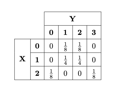
The values derived in Example 2.1.1 are the values taken by a joint probability mass function for two discrete random variables:

Let $X$ and $Y$ be two discrete random variables. The joint probability mass function (joint PMF) of $X$ and $Y$ is defined as

$p_{X,Y}(x,y) = P(X=x,Y=y).$

Note the probability values in Example 2.1.1 sum to $1$. This is because the collection of outcomes cover all possibilities. This is a property that is shared by all joint probability mass functions.

In this same vein, for some fixed outcome $x$ of $X$ one can calculate $P(X=x)$ from the joint PMF by summing the probabilities $P(X=x,Y=y)$ for all possible outcomes $y$ of $Y$: this collection of outcomes cover all possible scenarios in which $X=x$. A argument holds to calculate $p_Y(y)$. This argument is stated mathematically by the following lemma:

Joint PMFs can be used to calculate the PMFs of its random variables. Specifically $$\begin{align*} p_{X}(x) &= P(X=x)= \sum\limits_{y} P(X=x,Y=y), \\[3pt] p_Y(y) &= P(Y=y)= \sum\limits_{x} P(X=x,Y=y). \end{align*}$$

In this context, $p_X(x)$ and $p_{Y}(y)$ are called marginal PMFs.

Consider the three coin flips in Example 2.1.1. What is the probability that there is exactly one head observed?

Using the notation of Example 2.1.1, calculate via Lemma 1.1.3 that

$$\begin{align*} p_Y(1) &= P(Y=1) \\[3pt] &= P(X=0, Y=1) + P(X=1, Y=1) + P(X=2, Y=1) + P(X=3, Y=1) \\[3pt] &= 0 + \frac{1}{4} + \frac{1}{4} + 0 \\[3pt] &=\frac{1}{2}. \end{align*}$$

The following app allows the user to calculate the probabilities of both marginal PMFs of the coin flip problem outlined in Example 2.1.1.

Alternative to discrete random variables are continuous random variables: random variables which take values in some given range, rather than from some given set. We are already familiar with probability density functions, the analogous concent for continuous random variables to the probability mass function for discrete random variables. This is no different in the joint random variables case.

For any $(x,y)$ in $\mathbb{R}^2$, the probability $P(X=x,Y=y)$ is zero. Therefore the joint probability density function is not defined at individual points in $\mathbb{R}^{2}$, and is instead defined over regions in $\mathbb{R}^2$.

Let $X$ and $Y$ be continuous random variables. The joint probability density function (joint PDF) of $X$ and $Y$ is a function $f_{X,Y}$ with the property that for all $C \subset \mathbb{R}^{2}$:

$P \big( (x,y) \text{ in } C \big) = \iint_{C} f_{X,Y}(x,y) \,dx \,dy.$

Abbie and Bertie are playing a game in which they aim to score as many as they can. Abbie scores $X$, and Bertie scores $Y$. Although we are not fully aware of the rules for the game, we do know the joint PDF of $X$ and $Y$ is $$f_{X,Y}(x,y) = \begin{cases} 24x(1-x-y),& \text{if } x,y \geq 0 \text{ and } x+y \leq 1, \\ 0,& \text{otherwise.} \end{cases}$$ Calculate the probability that Abbie beats Bertie.

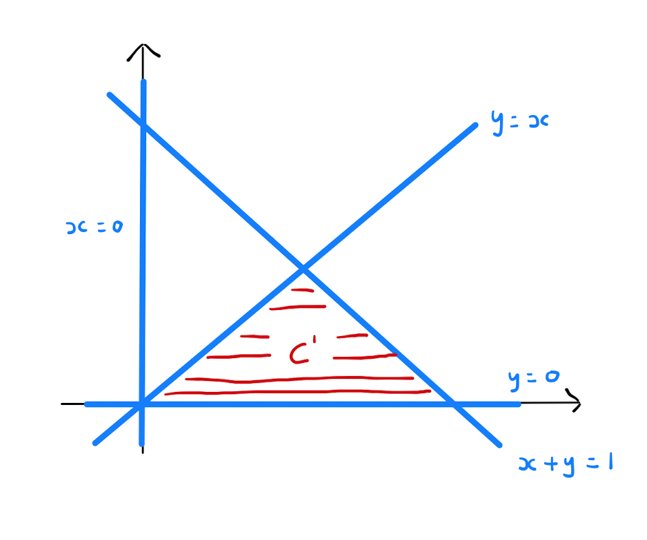
The problem is interpreted mathematically as calculating the probability $P(X>Y)$. Using Definition 2.1.5, this is akin to calculating the integral $\iint_{C} f_{X,Y}(x,y) \,dx\,dy$ where $C$ is the region in which $X>Y$. Since any integral of the constant function $0$ evaluates to $0$, we only need to consider the parts of $C$ that are contained within the region where $f_{X,Y}(x,y)$ is non-zero, that is, $\left\{ (x,y): x,y \geq 0 \text{ and } x+y \leq 1 \right\}$. Therefore the region $C'$ over which we will integrate is bounded by the lines $x=y$, $x+y=1$, $x=0$ and $y=0$.

Therefore

$$\begin{align*} P(X>Y) &= \int \int_{C} f_{X,Y}(x,y) \,dx\,dy \\[3pt] &= \int \int_{C'} 24x(1-x-y) \,dx\,dy \\[3pt] &= \int_{0}^{\frac{1}{2}} \int_{y}^{1-y} 24x-24x^2-24xy \,dx\,dy \\[3pt] &= \int_{0}^{\frac{1}{2}} \left[ 12x^2 - 8x^3 -12 x^2 y \right]_{y}^{1-y} \,dy \\[3pt] &= \int_{0}^{\frac{1}{2}} \left( 12 (1-y)^2 -8(1-y)^3 -12(1-y)^2 y \right) - \left( 12y^2 - 8y^3 -12y^3 \right) \,dy \\[3pt] &= \int_{0}^{\frac{1}{2}} 16y^3 -12y +4 \,dy \\[3pt] &= \left[ 4y^4 -6y^2 +4y \right]_{0}^{\frac{1}{2}} \\[3pt] &= \left( \frac{4}{16} - \frac{6}{4} +2 \right) - \left( 0 \right) \\[3pt] &= \frac{3}{4}. \end{align*}$$

Given a joint PDF, we can write R code them returns samples from the joint distribution. The following R code calculates $10000$ samples from the joint PDF $$f_{X,Y}(x,y) = \begin{cases} 6x^2y, & \text{if } 0 \leq x,y \leq 1, \\ 0, & \text{otherwise.} \end{cases}$$ Note that the region on which this joint PDF is non-zero is rectangular.

The code works by generating $50000$ points in the region on which $f_{X,Y}(x,y)$ is non-zero. These points are then chosen with probabilities governed by $f_{X,Y}(x,y)$. The samples are stored in the random variable `random_sample’.

#Create a 50000 points in the rectangle [0,1] x [0,1]
xs <- runif(50000, 0, 1)
ys <- runif(50000, 0, 1)
dat <- matrix(c(xs, ys), ncol = 2)
dat <- data.frame(dat)
names(dat) <- c("x", "y")

#Code to simulate the joint PDF
joint_pdf <- function(x, y) {
  6*x^2*y
}

#Evaluate the PDF at each of our 50000 points
probs <- joint_pdf(xs, ys)

#Choose 10000 samples from our 50000 points with probabilities governed by the PDF
indices <- sample(1:50000, 10000, replace=TRUE, prob=probs)
random_sample <- dat[indices, ]

It is also possible to write R code that takes samples from a joint PDF where the region on which the function is non-zero is not rectangular. Note the joint PDF governing the game played by Annie and Bertie in Example 2.1.6 is non-zero on a triangular region. The following R code calculates $10000$ samples from this joint PDF. The code is similar to that above with the sole difference being in the section defining the variable `joint_pdf’.

#Create a 50000 points in the rectangle [0,1] x [0,1]
xs <- runif(50000, 0, 1)
ys <- runif(50000, 0, 1)
dat <- matrix(c(xs, ys), ncol = 2)
dat <- data.frame(dat)
names(dat) <- c("x", "y")

#Code to simulate the joint PDF
joint_pdf <- function(x, y) {
  ifelse(x+y<1, 24*x*(1-x-y), 0) 
}

#Evaluate the PDF at each of our 50000 points
probs <- joint_pdf(xs, ys)

#Choose 10000 samples from our 50000 points with probabilities governed by the PDF
indices <- sample(1:50000, 10000, replace=TRUE, prob=probs)
random_sample <- dat[indices, ]

Crucially by taking sufficiently large samples, one can estimate probabilities related to the joint PDF. The following R code verifies the solution to Example 2.1.6 by estimating $P(X>Y)$ using the variable `random_sample’ defined in the prior block.

mean(random_sample$x > random_sample$y)

While R is useful for plotting and working with random samples, it is not good for working with symbolic mathematics.

Similarly to the discrete case, the PDF of $X$ can be recovered from the joint PDF by totaling $f_{X,Y}(x,y)$ across all possible values of $y$ for $Y$. This is stated mathematically by the following lemma.

Joint PDFs can be used to calculate the PDFs of its random variables. Specifically $$\begin{align*} f_{X}(x) &= \int_{-\infty}^{\infty} f_{X,Y}(x,y) \,dy, \\[3pt] f_Y(y) &= \int_{-\infty}^{\infty} f_{X,Y}(x,y) \,dx. \end{align*}$$

In this context, $f_X(x)$ and $f_{Y}(y)$ are called marginal PDFs.

Consider the game from Example 2.1.6. Calculate the marginal PDF of Abbie’s score.

The question asks us to calculate $f_{X}(x)$. Since $f_{X,Y}(x,y)$ is $0$ for all $x<0$ and $x>1$, it is enough for us to consider $0 \leq x \leq 1$. By Lemma 2.1.7, calculate

$$\begin{align*} f_{X}(x) &= \int_{-\infty}^{\infty} f_{X,Y}(x,y) \,dy \\[3pt] &= \int_{0}^{1-x} 24x(1-x-y) \,dy \\[3pt] &= \left[ -12x(1-x-y)^2 \right]_{0}^{1-x} \\[3pt] &= 12x(1-x)^2. \end{align*}$$

Therefore

$f_{X}(x) = \begin{cases} 12x(1-x)^2, & \text{if } 0 \leq x \leq 1, \\[3pt] 0, & \text{otherwise.} \end{cases}$

2.2 Joint cumulative distribution functions

There are two random variables that we are concerned about in the F1 racing problem: namely the time $X$ that Max Verstappen sets and the time $Y$ that Sergio Perez sets. It follows that

$$P \big(\text{Hamilton not on the front row} \big) = P \big( X \leq 1:11.116, Y \leq 1:11.116 \big)$$

Probabilities where two random variables are both less than some fixed values are a well-studied phenomenon in probability.

The joint cumulative distribution function of two random variables $X$ and $Y$ is defined by

$$F_{X,Y}(x,y) = P(X \leq x, Y \leq y).$$

Two friends are meeting in Nottingham city center. Both travel via buses on different routes that come once an hour. Let $X$ and $Y$ be the time, as a proportion of an hour, until the respective buses come. The joint cumulative distribution function is $$F_{X,Y}(x,y) = xy, \qquad \text{where } 0 \leq x,y \leq 1.$$ What is the probability that both friends are on a bus to Nottingham within half an hour?

Since we want both buses to arrive within half an hour, we want the probability that $X \leq \frac{1}{2}$ and $Y \leq \frac{1}{2}$. Calculate

$$\begin{align*} P \left( X \leq \frac{1}{2}, Y \leq \frac{1}{2} \right) &= F_{X,Y} \left( \frac{1}{2}, \frac{1}{2} \right) \\[3pt] &= \frac{1}{2} \cdot \frac{1}{2} \\[3pt] &= \frac{1}{4}. \end{align*}$$

In general we would like to define $F_{X,Y}(x,y)$ on all of $\mathbb{R}^{2}$, that is, $X$ and $Y$ can take any real number value. Consider the cumulative distribution function from Example 2.1.2.

Given a joint CDF $F_{X,Y}$, the CDF for $X$ and $Y$, denoted $F_X, F_Y$ and in this context called marginal CDFs, can be calculated. Specifically

$$\begin{align*} F_X(x) = F_{X,Y} (x,\infty) \\[3pt] F_Y(y) = F_{X,Y} (\infty, y) \end{align*}$$

Intuitively this lemma makes sense: $P(X<x, Y< \infty) = P(X<x)$ since $Y$ being less than $\infty$ will always be true.

Consider the buses of Example 2.2.2. Calculate the marginal CDF of both buses.

Since the problem is entirely symmetrical when interchanging $x$ and $y$ it is enough to only calculate $F_X(x)$. For $0\leq x \leq 1$, by Lemma 2.2.3 we have that

$$\begin{align*} F_{X}(x) &= F_{X,Y}(x,\infty) \\[3pt] &= F_{X,Y}(x,1) \\[3pt] &= x. \end{align*}$$ It follows by the aforementioned symmetry that $F_Y(y) = y$ for $0 \leq y \leq 1$.

In Definition 2.2.1, we saw that $F_{X,Y}(x,y) = P \left( X \leq x, Y \leq y \right)$. However by Definition 2.1.5, we also have that $P \left( X \leq x, Y \leq y \right) = \int_{-\infty}^{y} \int_{-\infty}^{x} f_{X,Y}(u,v) \,du \,dv$. Therefore

$$F_{X,Y}(x,y) = \int_{-\infty}^{y} \int_{-\infty}^{x} f_{X,Y}(u,v) \,du \,dv.$$

Taking the second order derivative of this equation, differentiating with respect to $x$ and $y$, we obtain:

$$f_{X,Y}(x,y) = \frac{\partial^2 F_{X,Y}(x,y)}{\partial x \partial y}.$$

These equations give us a method to calculate the joint PDF from the joint CDF, and vice-versa.

Consider the buses of Example 2.2.2, the arrival times of which are governed by the joint CDF $$F_{X,Y}(x,y) = xy, \qquad \text{where } 0 \leq x,y \leq 1.$$ Calculate the joint PDF of the bus arrival times.

By the above theory, for $0\leq x,y \leq 1$ calculate that $$\begin{align*} f_{X,Y}(x,y) &= \frac{\partial^2 F_{X,Y}(x,y)}{\partial x \partial y} \\ &= \frac{\partial^2}{\partial x \partial y} \left( xy \right) \\ &= \frac{\partial}{\partial x} \left( x \right) \\ &= 1. \end{align*}$$ So $f_{X,Y}=1$ when $0\leq x,y \leq 1$.

2.3 Independence

When considering two events, it can be tempting to calculate the probability of the desired outcome for both events and then multiply these probabilities together. But what if the two events are not independent? Then this argument breaks down.

In the F1 racing example, Max Verstappen and Sergio Perez both drive in cars designed by the Red Bull racing team. If one of the drivers is slow because of a deficiency in the car, then the other driver may also record a slow time because of the same deficiency. Alternatively if one driver posts a fast time because of an outstanding car, then it is perhaps more likely that the other driver will be similarly fast. The two lap times are not independent.

Recall that two events $A$ and $B$ are independent if $P(A \cap B) = P(A) P(B)$. The notion of independence of events can be extended to a notion of independence of random variables.

The random variables $X$ and $Y$ with PDFs $f_X$ and $f_y$ respectively, are said to be independent if $$f_{X,Y}(x,y) = f_{X}(x) f_{Y}(y),$$ for all values of $x$ and $y$.

The condition $F_{X,Y}(x,y) = F_{X}(x) F_{Y}(y)$ in Definition 2.3.1 is equivalent to the condition $$P(X \leq x, Y \leq y) = P(X \leq x)\cdot P(Y\leq y).$$

The following theorem allows us to check independence of two random variables from PDFs instead of CDFs.

Suppose the CDF $F_{X,Y}(x,y)$ is differentiable. Then jointly continuous random variables $X$ and $Y$ are independent if and only if $$f_{X,Y}(x,y) = f_{X}(x) f_{Y}(y),$$ for all values of $x$ and $y$.

Specifically given two random variables $X$ and $Y$ with joint PDF $f_{X,Y}(x,y)$, one can check independence by calculating both marginal PDFs $f_{X}(x)$ and $f_{Y}(y)$, then applying Theorem 2.3.2.

Consider again the game played by Abbie and Bertie in Example 2.1.6, the scores of which are governed by the joint PDF $$f_{X,Y}(x,y) = \begin{cases} 24x(1-x-y),& \text{if } x,y \geq 0 \text{ and } x+y \leq 1, \\ 0,& \text{otherwise.} \end{cases}$$ Are the scores of Abbie and Bertie independent?

Recall from Example 2.1.8 that Abbies’ score is distributed by the marginal PDF

$$f_{X}(x) = \begin{cases} 12x(1-x)^2, & \text{if } 0 \leq x \leq 1, \\ 0, & \text{otherwise.} \end{cases}$$

Calculating the marginal PDF of Berties’ score for $0\leq y \leq 1$:

$$\begin{align*} f_{Y}(y) &= \int_{-\infty}^{\infty} f_{X,Y}(x,y) \,dx \\[3pt] &= \int_{0}^{1-y} 24x(1-x-y) \,dx \\[3pt] &= \int_{0}^{1-y} 24x-24x^2-24xy \,dx \\[3pt] &= \left[ 12x^2 -8x^3 -12x^2 y \right]_{0}^{1-y} \\[3pt] &= 12(1-y)^2 - 8(1-y)^3 -12 (1-y)^2 y \\[3pt] &= 4(1-y)^3. \end{align*}$$

Therefore

$$f_{Y}(y) = \begin{cases} 4(1-y)^3, & \text{if } 0 \leq y \leq 1, \\ 0, & \text{otherwise.} \end{cases}$$

Immediately one can see that $f_{X,Y}(x,y) \neq f_{X}(x) f_{Y}(y)$: for example $f_{X,Y} \left(\frac{3}{4}, \frac{3}{4} \right) = 0$ since $\frac{3}{4} + \frac{3}{4} > 1$, but $f_{X} \left( \frac{3}{4} \right) f_{Y} \left( \frac{3}{4} \right) = \frac{9}{16} \cdot \frac{1}{16} = \frac{3}{16^2}$.

Therefore Abbie and Berties’ scores are dependent.

Consider again the buses of Example 2.2.2, the arrival times of which are governed by the joint CDF $$F_{X,Y}(x,y) = xy, \qquad \text{where } 0 \leq x,y \leq 1.$$ Are the arrival times of the buses independent?

In Example 2.2.4, we calculated the marginal distributions $F_X (x) = x$ for $0 \leq x \leq 1$ and $F_Y (y) = y$ for $0 \leq y \leq 1$. It follows that

$$F_{X,Y}(x,y) = xy = F_{X}(x) F_{Y}(y).$$ Therefore the bus arrival times are independent.

2.4 Three or more random variables

All the ideas and notions seen in this chapter can be extended to the setting of more than two random variables.

Specifically let $n$ be a positive integer with $n \geq 2$. Consider $n$ random variables denoted $X_1,X_2, \ldots, X_n$. Then

• assuming $X_1,X_2, \ldots, X_n$ are discrete, the joint PMF of $X_1,X_2 \ldots, X_n$ is a function $p_{X_1,X_2 \ldots, X_n}$ such that $$p_{X_1,X_2 \ldots, X_n}(x_1,\ldots,x_n) = P(X_1 =x_1, \ldots , X_n=x_n);$$

• the joint CDF of $X_1,X_2 \ldots, X_n$ is a function $F_{X_1,X_2 \ldots, X_n}$ such that
  $$F_{X_1,X_2 \ldots, X_n}(x_1,x_2 \ldots, x_n) = P \left( X_1 \leq x_1, X_2 \leq x_2 \ldots , X_n \leq x_n \right);$$

• assuming $X_1,X_2, \ldots, X_n$ are continuous, the joint PDF of $X_1,X_2 \ldots, X_n$ is the function $f_{X_1,X_2 \ldots, X_n}(x_1,x_2 \ldots, x_n)$ such that for any region $C \subseteq \mathbb{R}^{n}$, the probability $$P \big( \left(X_1, X_2, \ldots, X_n \right) \in C \big) = \int \cdots \int_{C} f_{X_1,X_2 \ldots, X_n}(x_1,x_2 \ldots, x_n) \,dx_1 \cdots \,dx_n;$$

• assuming $X_1,X_2, \ldots, X_n$ are continuous, the joint PDF $f_{X_1,X_2 \ldots, X_n}(x_1,x_2 \ldots, x_n)$ and joint CDF $F_{X_1,X_2 \ldots, X_n}(x_1,x_2 \ldots, x_n)$ are related by the identity $$f_{X_1,X_2 \ldots, X_n}(x_1,x_2 \ldots, x_n) = \frac{\partial^n F_{X_1,X_2 \ldots, X_n}(x_1,x_2 \ldots, x_n)}{\partial x_1 \ldots \partial x_n};$$

• the marginal CDF of $X_i$ for $1 \leq i \leq n$ can be obtained by substitution into the joint CDF: $$F_{X_i}(x_i) = F_{X_1,X_2 \ldots, X_n}(\infty, \infty, \ldots, \infty, x_i, \infty, \ldots, \infty);$$

• assuming $X_1,X_2, \ldots, X_n$ are continuous, the marginal PDF of $X_i$ for $1\leq i \leq n$ can be obtained by integration of the joint PDF: $$f_{X_i}(x_i) = \int \cdots \int_{\mathbb{R}^{n-1}} f_{X_1,X_2 \ldots, X_n}(x_1,x_2 \ldots, x_n) \,dx_1 \,dx_2 \ldots \,dx_{i-1} \,dx_{i+1} \ldots \,dx_n;$$

• the random variables $X_1, X_2, \ldots , X_n$ are said to be independent if $$F_{X_1,X_2 \ldots, X_n}(x_1,x_2 \ldots, x_n) = F_{X_1}(x_1) F_{X_2}(x_2) \cdots F_{X_n}(x_n).$$

Compare all of the statements here with the analogous definitions earlier in the chapter when two random variables were considered. In particular set $n=2$ in each bullet point to recover an earlier definition or lemma.

2.5 Expectation

Norwegian Air run a small five person passenger plane from Oslo to Nordfjordeid. In order to analyse future financial prospects, the company would like to understand fuel consumption of the flight. To calculate fuel consumption, Norwegian air needs to know the total weight of the five passengers. Obviously this quantity will change from flight-to-flight, and so Norwegian Air will have to calculate an expected value for the total weight.

The next flight has a family of $5$ booked on: a male parent, a female parent and three teenage children. Norwegian air know that the weight of an adult male is modeled by a continuous random variable $W_{\text{adult male}}$. Similarly $W_{\text{adult male}}$ is a continuous random variable that models the weight of an adult female and $W_\text{teenager}$ is a random variable that models the weight of a teenager. Norwegian Air would therefore like to predict the average value of $W_{\text{adult male}} + W_{\text{adult female}} + 3 W_\text{teenager}$, that is $\mathbb{E}\left[W_{\text{adult male}} + W_{\text{adult female}} + 3 W_\text{teenager} \right]$.

More generally, given a collection of continuous random variables $X_1, \ldots, X_n$, what is the expected value of some function $g \left( X_1, \ldots, X_n \right)$ of these random variables.

In MATH1055, we saw the solution to the analogous discrete problem with $n=2$: how to calculate the expectation of a function of two discrete random variables.

Let $X_1$ and $X_2$ be two discrete random variables, with joint PMF denoted $p_{X_1,X_2}$. Then, for a function of the two random variables $g(X_1,X_2)$, we have $$\mathbb{E}[g(X_1,X_2)] = \sum_{(x_1,x_2)} g(x_1,x_2) p_{X_1,X_2}(x_1,x_2).$$

In Theorem 2.5.1, the summation is over all pairs of values $x_1, x_2$ that $X_1, X_2$ can take respectively. Since the term inside the summation involves $p_{X_1,X_2}(x_1,x_2)$, it is enough to only consider pairs $(x_1,x_2)$ for which $p_{X_1,X_2}(x_1,x_2) \neq 0$, that is, only the pairs that have a change of occurring.

A cafe wants to investigate the correlation between temperature $X$ in degrees Celsius during winter and the number of customers $Y$ in the cafe each day. Based on existing data collected by the owner, the joint probability table is

What is the average number of customers per day?

In mathematical language, the question is asking us to calculate $\mathbb{E}\left[ Y \right]$. Setting $g(X,Y) = Y$, by Theorem 2.5.1: $$\begin{align*} \mathbb{E}\left[ Y \right] &= \sum_{(x,y)} g(x,y) p_{X,Y}(x,y) \\[5pt] &= 15 \cdot p_{X,Y}(0,15) + 75 \cdot p_{X,Y}(0,75) + 150 \cdot p_{X,Y}(0,150) \\ &\qquad + 15 \cdot p_{X,Y}(10,15) + 75 \cdot p_{X,Y}(10,75) + 150 \cdot p_{X,Y}(10,150) \\ & \qquad \qquad + 15 \cdot p_{X,Y}(20,15) + 75 \cdot p_{X,Y}(20,75) + 150 \cdot p_{X,Y}(20,150) \\[5pt] &= (15 \times 0.07 ) + ( 75 \times 0.11) + (150 \times 0.01) \\ &\qquad + (15 \times 0.23) + (75 \times 0.43) + (150 \times 0.05) \\ & \qquad \qquad + (15 \times 0.04) + (75 \times 0.05) + (150 \times 0.01) \\[5pt] &= 58.35 \end{align*}$$

Theorem 2.5.1 generalises to considering three or more variables. This is possible due to the introduction of joint PMFs in Section 2.4.

Let $X_1, \ldots, X_n$ be a collection of discrete random variables, with joint PMF denoted $p_{X_1, \ldots, X_n}$. Then, for a function of the random variables $g(X_1,\ldots, X_n)$, we have $$\mathbb{E}[g(X_1,\ldots, X_n)] = \sum_{(x_1,\ldots, x_n)} g(x_1,\ldots , x_n) p_{X_1,\ldots, X_n}(x_1,\ldots, x_n).$$

The generalisation of Theorem 2.5.3 to the case of continuous random variables involves integrating over the continuous region of possibilities, rather than summing over the discrete collection of possibilities.

Let $X_1, \ldots, X_n$ be a collection of continuous random variables, with joint PDF denoted $f_{X_1, \ldots, X_n}$. Then, for a function of the random variables $g(X_1 \ldots, X_n)$, we have $$\mathbb{E}[g(X_1,\ldots, X_n)] = \int_{-\infty}^{\infty} \cdots \int_{-\infty}^{\infty} g(x_1,\ldots , x_n) f_{X_1,\ldots, X_n}(x_1,\ldots, x_n) \,dx_1 \cdots \,dx_n.$$

Consider two random variables with joint PDF given by $$f_{X,Y}(x,y) = \begin{cases} 2(x+y), & \text{if } 0 \leq x \leq y \leq 1, \\ 0, & \text{otherwise.} \end{cases}$$ Calculate the expected value of $XY$.

The two-dimensional region on which $f_{X,Y}(x,y)$ is non-zero is

By applying Theorem 2.5.4, we have that $$\begin{align*} \mathbb{E}[XY] &= \int_{-\infty}^{\infty} \int_{-\infty}^{\infty} xy \cdot f_{X,Y}(x,y) \,dx \,dy \\[3pt] &= \int_0^1 \int_0^y xy \cdot 2(x+y) \,dx \,dy \\[3pt] &= \int_0^1 \int_0^y 2x^2y + 2x y^2 \,dx \,dy \\[3pt] &= \int_0^1 \left[ \frac{2}{3}x^3 y + x^2 y^2 \right]_0^y \,dy \\[3pt] &= \int_0^1 \frac{2}{3} y^4 + y^4 \,dy \\[3pt] &= \int_0^1 \frac{5}{3} y^4 \,dy \\[3pt] &= \left[ \frac{1}{3} y^5 \right]_0^1 \\[3pt] &= \frac{1}{3}. \end{align*}$$

2.6 Covariance

Consider two random variables $X$ and $Y$. We have seen the notion of independence: $X$ and $Y$ have no impact on each other. Alternatively there could exist a positive relationship, that is as one of $X,Y$ increases so does the other, or an inverse relationship, as one of $X,Y$ increases the other decreases and vice-versa.

The mathematical quantities of covariance studied in this section, and correlation studied in Section 2.7 identify any such relationship and measures its strength.

The covariance of two random variables, $X$ and $Y$, is defined by

$$\text{Cov}(X,Y) = E\Big[(X-E[X])(Y-E[Y])\Big]$$

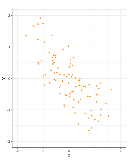
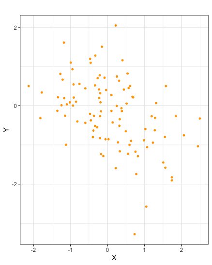
If $\text{Cov}(X,Y)$ is positive, both random variables generally tend to be large and small at the same time. If $\text{Cov}(X,Y)$ is negative, then as one random variable is large the other tends to be small. The strength of any such relationship between $X$ and $Y$ is not accounted for by the covariance.

Scatter plots of samples taken from random variables $X$ and $Y$ with positive covariance
               

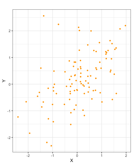
Scatter plots of samples taken from random variables $X$ and $Y$ with negative covariance
               

There is a simpler formula than that of Definition 2.6.1 by which to calculate covariance. Specifically it can be shown that covariance is equal to the expected value of the product minus the product of the expected values.

The covariance of two random variables, $X$ and $Y$, can by calculated by $$\text{Cov}(X,Y) = E[XY]-E[X]E[Y].$$

Calculate the covariance of the random variables $X, Y$ in Example 2.5.2 that govern the temperature and number of customers daily in the cafe.

Motivated by the formula $\text{Cov}(X,Y) = E[XY]-E[X]E[Y]$ for covariance, we seek to calculate $E[X], E[Y]$ and $E[XY]$. From Example 2.5.2, we know $E[Y] = 58.35$. Now calculating $E[X]$ and $E[XY]$ using Theorem 2.5.4, obtain

$$\begin{align*} E[X] &= 0 \times P(X=0) + 10 \times P(X=10) + 20 \times P(X=20) \\[3pt] &= 0 \times (0.07 + 0.11 + 0.01) + 10 \times (0.23 + 0.43 + 0.05) + 20 \times (0.04 + 0.05 + 0.01) \\[3pt] &= 9.1, \\[9pt] E[XY] &= \sum\limits_{n \in \mathbb{Z}} n \cdot P(XY =n) \\[3pt] &= \sum\limits_{\begin{array}{c} n=-\infty \\ n: \text{ integer} \end{array}}^{\infty} n \cdot P(XY =n) \\[3pt] &= 0 \times \big( p_{X,Y}(0,15) + p_{X,Y}(0,75) + p_{X,Y}(0,150) \big) + 150 \times p_{X,Y}(10,15) + 300 \times p_{X,Y}(20,15) \\ &\qquad \qquad + 750 \times p_{X,Y}(10,75) + 1500 \times \big( p_{X,Y}(10,150) + p_{X,Y}(20,75) \big) + 3000 \times p_{X,Y}(20,150) \\[3pt] &= 0 \times \left( 0.07 + 0.11 + 0.01 \right) + 150 \times 0.23 + 300 \times 0.04 + 750 \times 0.43 \\ & \qquad \qquad + 1500 \times \left( 0.05 + 0.05 \right) + 3000 \times 0.01 \\[3pt] &= 549. \end{align*}$$

Therefore it follows that

$$\text{Cov}(X,Y) = 549 - 9.1 \times 58.35 = 18.015.$$

Calculate the covariance of the random variables $X, Y$ in Example 3.1.5.

Again we seek to apply the formula $\text{Cov}(X,Y) = E[XY]-E[X]E[Y]$. From Example 2.5.5, we know $E[XY] = \frac{1}{3}$. Calculating $E[X]$ and $E[Y]$ using Theorem 2.5.4, obtain

$$\begin{align*} E[X] &= \int_{-\infty}^{\infty} \int_{-\infty}^{\infty} x \cdot f_{X,Y}(x,y) \,dx \,dy \\[3pt] &= \int_0^1 \int_0^y 2x(x+y) \,dx \,dy \\[3pt] &= \int_0^1 \int_0^y 2x^2 + 2xy \,dx \,dy \\[3pt] &= \int_0^1 \left[ \frac{2}{3}x^3 + x^2 y \right]_0^y \,dy \\[3pt] &= \int_0^1 \frac{2}{3}y^3 + y^3 \,dy \\[3pt] &= \int_0^1 \frac{5}{3} y^3 \,dy \\[3pt] &= \left[ \frac{5}{12}y^4 \right]_0^1 \\[3pt] &= \frac{5}{12}, \\[9pt] E[Y] &= \int_{-\infty}^{\infty} \int_{-\infty}^{\infty} y \cdot f_{X,Y}(x,y) \,dx \,dy \\[3pt] &= \int_0^1 \int_0^y 2y(x+y) \,dx \,dy \\[3pt] &= \int_0^1 \int_0^y 2xy+2y^2 \,dx \,dy \\[3pt] &= \int_0^1 \left[ x^2 y + 2xy^2 \right]_0^y \,dy \\[3pt] &= \int_0^1 y^3 + 2y^3 \,dy \\[3pt] &= \int_0^1 3y^3 \,dy \\[3pt] &= \left[ \frac{3}{4}y^4 \right]_0^1 \\[3pt] &= \frac{3}{4}. \end{align*}$$

Therefore it follows that

$$\text{Cov}(X,Y) = \frac{1}{3} - \frac{5}{12}\cdot \frac{3}{4} = \frac{1}{48}.$$

The covariance of two sample populations can be calculated in R. The following code calculates the covariance of a known sample of size $5$ taken from two random variables $X$ and $Y$:

X_samp = c(3,4,7,8,10) 
Y_samp = c(1,21,3,13,15)
cov(X_samp,Y_samp)

Covariance has the following important properties:

• If $X$ and $Y$ are independent, then $\text{Cov}(X,Y) = 0$. However if $\text{Cov}(X,Y) = 0$, then $X$ and $Y$ do not necessarily have to be independent;

• The covariance of two equal random variables is equal to the variance of that random variable. $$\text{Cov}(X,X) = \text{Var}(X);$$

• There is a further relationship between variance and covariance: $$\text{Var}(X+Y) = \text{Var}(X) + \text{Var}(Y) + 2\text{Cov}(X,Y).$$ That is to say, that covariance describes the variance of the random variable $X+Y$ that is not explained by the variances of the random variables $X$ and $Y$;

• More generally the above relationship between variance and covariance generalises to: $$\text{Var} \left( \sum_{i=1}^n a_iX_i \right) = \sum_{i=1}^n a_i^2 \text{Var}(X_i) + 2 \sum_{1 \leq i < j \leq n} a_ia_j\text{Cov}(X_i,X_j);3$$

• Assume that $X_1,X_2,\dots,X_n$ are independent so that $\text{Cov}(X_i,X_j)=0$, and also assume that each $a_i$ is equal to $1$. This derives the formula: $$\text{Var} \left( \sum_{i=1}^n X_i \right) = \sum_{i=1}^n \text{Var} (X_i).$$

Suppose $X$ and $Y$ are discrete random variables whose probability mass function is given by the following table:

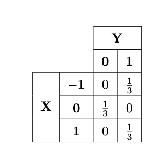
What is the covariance of the two variables? Are they independent?

From the table, one can calculate the probability mass functions for $X$ and $Y$:

$$p_{X} (x) = \begin{cases} \frac{1}{3}, & \text{if } x=-1 \\[5pt] \frac{1}{3}, & \text{if } x=0 \\[5pt] \frac{1}{3}, & \text{if } x=1 \end{cases}$$ and $$p_{Y} (y) = \begin{cases} \frac{1}{3}, & \text{if } y=0 \\[5pt] \frac{2}{3}, & \text{if } y=1 \end{cases}$$

Using $p_{X}, p_{Y}$ and $p_{X,Y}$, we can calculate the expectation of $X$, $Y$ and $XY$ respectively:

$$\begin{align*} E[X] &= \sum\limits_{x} x \cdot p_{X}(x) \\ &= \left( -1 \times \frac{1}{3} \right) + \left( 0 \times \frac{1}{3} \right) + \left( 1 \times \frac{1}{3} \right) \\ &= 0 \\[9pt] E[Y] &= \sum\limits_{y} y \cdot p_{Y}(y) \\ &= \left( 0 \times \frac{1}{3} \right) + \left( 1 \times \frac{2}{3} \right) \\ &= 2/3 \\[9pt] E[XY] &=\sum\limits_{(x,y)} x \cdot y \cdot p_{X,Y}((x,y) ) \\ &= \left( -1 \times 0 \times 0 \right) + \left( 0 \times 0 \times \frac{1}{3} \right) + \left( 1 \times 0 \times 0 \right) \\ & \qquad \qquad + \left( -1 \times 1 \times \frac{1}{3} \right) + \left( 0 \times 1 \times 0 \right) + \left( 1 \times 1 \times \frac{1}{3} \right) \\ &= 0 \\ \end{align*}$$

The covariance can then be calculated using Definition 2.6.1:

$$\begin{align*} \text{Cov}(X,Y) &= E[XY] - E[X]E[Y] \\ &= 0-0 \\ &= 0. \end{align*}$$

This does not inform us whether $X$ and $Y$ are independent or not. However, note that

$$p_{X,Y}(0,0) = \frac{1}{3} \qquad \text{and} \qquad p_X(0) \cdot p_Y(0) = \frac{1}{3}\cdot \frac{1}{3} = \frac{1}{9}.$$ So $p_{X,Y}(0,0) \neq p_X(0)p_Y(0)$ and therefore, $X$ and $Y$ are not independent.

There are some rules which allow us to easily calculate the covariance of linear combinations of random variables.

Let $a,b$ be real numbers, and $X,X_1, X_2, Y, Y_1, Y_2$ be random variables. Each of the following rules pertaining to covariance hold in general

$$\begin{align*} \text{Cov}(X+a,Y+b) &= \text{Cov}(X,Y) \\[5pt] \text{Cov}(aX,bY) &= ab\text{Cov}(X,Y) \\[5pt] \text{Cov}(X_1+X_2,Y_1+Y_2) &= \text{Cov}(X_1,Y_1) + \text{Cov}(X_1,Y_2) \\ & \qquad + \text{Cov}(X_2,Y_1) + \text{Cov}(X_2,Y_2) \\[5pt] \end{align*}$$

Consider the cafe from Example 2.5.2. Calculate the covariance of the number of customers the cafe receives in a three day and the average temperature over these three days in degrees Fahrenheit. You may assume that the values $X$ and $Y$ on any given day are independent of the values taken by $X$ and $Y$ on the other days.

In mathematical language, the total number of customers over a three day period can be modeled by $3X$. The average temperature in degrees Celsius is modeled by $\frac{1}{3} \big( Y + Y + Y \big) = \frac{1}{3} \big( 3Y \big) = Y$, which converting into degrees Fahrenheit is $\frac{9}{5}Y + 32$. Therefore we aim to calculate $\text{Cov}\left( 3X,\frac{9}{5}Y + 32 \right)$. Applying Lemma 2.6.6 and using the result of Example 2.6.3, obtain

$$\text{Cov}\left( 3X,\frac{9}{5}Y + 32 \right) = 3\cdot \frac{9}{5} \cdot \text{Cov}(X,Y) = 3 \times 1.8 \times 18.015 = 97.281.$$

2.7 Correlation

Suppose two random variables have a large covariance. There are two factors that can contribute to this: the variance of $X$ and $Y$ as individual random variables could be high, that is the magnitude of $X - E[X]$ and $Y - E[X]$ are particularly large, or the relationship between $X$ and $Y$ could be strong. We would like to isolate this latter contribution.

By scaling covariance to account for the variance of $X$ and $Y$, one obtains a mathematical quantity, known as correlation, that solely tests the relationship between two random variables, and provides a measure of the strength of this relationship.

If $\text{Var}(X)>0$ and $\text{Var}(Y)>0$, then the correlation of $X$ and $Y$ is defined by

$$\rho(X,Y) = \frac{\text{Cov}(X,Y)}{\sqrt{\text{Var}(X)\text{Var}(Y)}}.$$

The correlation of two sample populations can be calculated in R. The following code calculates the correlation of a known sample of size $5$ taken from two random variables $X$ and $Y$:

X_samp = c(3,4,7,8,10) 
Y_samp = c(1,21,3,13,15)
cor(X_samp,Y_samp)

Correlation has the following important properties:

• $-1 \leq \rho(X,Y) \leq 1$;

• If $\rho(X,Y) = 1$, then there is a perfect linear positive correlation between $X$ and $Y$. If $\rho(X,Y) = -1$, then there is a perfect linear inverse correlation between $X$ and $Y$;

• If $X$ and $Y$ are independent, then $\rho(X,Y)=0$. Note, again, that the converse is not true.

These properties can be explored in the following app.

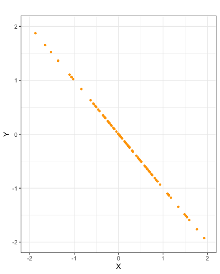
While a correlation $\rho(X,Y)=1$ indicates a perfect positive linear relationship between $X$ and $Y$, it is important to note that the correlation does not indicate the gradient of this linear relationship. Specifically an increase in $X$ does not indicate an equal increase in $Y$. A similar statement holds for correlation $\rho(X,Y)=-1$.

Scatter plots of samples taken from random variables $X$ and $Y$ with correlation $1$
               
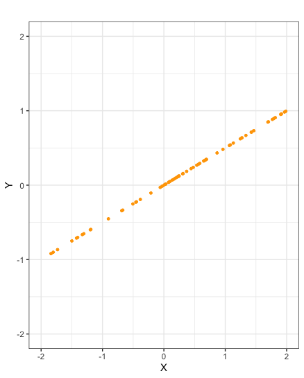
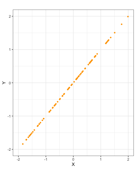
Scatter plots of samples taken from random variables $X$ and $Y$ with correlation $-1$
               

Similarly to covariance, there are identities that help us to calculate the correlation of linear combinations of random variables.

Let $a,b$ be real numbers, and $X,Y$ be random variables. Both of the following rules pertaining to correlation hold in general:

$$\begin{align*} \rho(X+a, Y+b) &= \rho(X,Y) \\[5pt] \rho (aX,bY) &= \begin{cases} \rho(X,Y), & \text{if } ab>0, \\[3pt] -\rho(X,Y), & \text{if } ab<0. \end{cases} \end{align*}$$

Let $X_i \sim Exp(\lambda_i)$ where $\lambda_i >0$ for $i=0,1,2$ be a collection of independent random variables. Set

$$\begin{align*} Y_1 &= X_0 + X_1 \\[3pt] Y_2 &= X_0 + X_2 \end{align*}$$

Calculate the correlation $\rho(Y_1,Y_2)$ of $Y_1$ and $Y_2$.

Calculate

$$\text{Var}(Y_1) = \text{Var}(X_0 + X_1) = \text{Var}(X_0) + \text{Var}(X_1) = \frac{1}{\lambda_0^2} + \frac{1}{\lambda_1^2}.$$

Similarly

$$\text{Var}(Y_2) = \frac{1}{\lambda_0^2} + \frac{1}{\lambda_2^2}.$$

Now

$$\begin{align*} \text{Cov}(Y_1,Y_2) &= \text{Cov}(X_0 + X_1, X_0 + X_2) \\[3pt] &= \text{Cov}(X_0,X_0) + \text{Cov}(X_1,X_0) + \text{Cov}(X_0,X_2) + \text{Cov}(X_1,X_2) \\[3pt] &= \text{Var}(X_0) + 0 + 0 + 0 \\[3pt] &= \frac{1}{\lambda_0^2}. \end{align*}$$

Therefore

$$\begin{align*} \rho(Y_1, Y_2) &= \frac{\text{Cov}(Y_1,Y_2)}{\sqrt{\text{Var}(Y_1)\text{Var}(Y_2)}} \\[5pt] &= \frac{ \frac{1}{\lambda_0^2} }{ \sqrt{ \left(\frac{1}{\lambda_0^2} + \frac{1}{\lambda_1^2} \right) \left(\frac{1}{\lambda_0^2} + \frac{1}{\lambda_2^2} \right)} } \\[5pt] &= \frac{\lambda_0^2 \lambda_1 \lambda_2 \cdot \frac{1}{\lambda_0^2} }{\lambda_0^2 \lambda_1 \lambda_2 \cdot \sqrt{ \left(\frac{1}{\lambda_0} + \frac{1}{\lambda_1} \right) \left(\frac{1}{\lambda_0} + \frac{1}{\lambda_2} \right)} } \\[5pt] &= \frac{\lambda_1 \lambda_2}{\sqrt{(\lambda_0^2 + \lambda_1^2)(\lambda_0^2 + \lambda_2^2)}}. \end{align*}$$