Chapter 8 Stochastic Process and Markov Chains

8.1 Strochastic Processes

A stochastic process is a family of random variables $\left\{ X_t: t \in T \right\}$ where the index $t$ belongs to some parameter set $T$, and each of the random variables can take the same set of possible values. The possible values that the random variables can take is known as the state space.

Typically the indices $t$ and parameter set $T$ have a time-related interpretation. With this in mind, informally a stochastic process can be thought of as the state of some system at a time $t$. When the set $T$ is discrete, for example $T=\{ 0,1,2,3,4,5,\ldots \}$, then the stochastic process $\left\{ X_t: t \in T \right\}$ is known as a discrete-time process. When the set $T$ is continuous, for example $T=[0, \infty)$, then the stochastic process $\left\{ X_t: t \in T \right\}$ is known as a continuous-time process. In DATA2002, we will predominantly consider stochastic processes that are discrete time processes.

Furthermore throughout the remainder of DATA2002, we will only consider stochastic processes for which the state space is discrete, that is, each of the $X_t$ are discrete random variables.

Consider a fair $6$-sided die that we roll repeatedly keeping track of our total cumulative score. Let $X_t$ be the total of the first $t$ dice rolls. What is the parameter set $T$, and what is the state space denoted $S$. Also calculate the PMFs of $X_1$ and $X_2$.

The index $t$ corresponds the number of dice rolls that have been made, and so will be a positive whole integer. Therefore $$T=\{ 1,2,3,4,5,\ldots \}.$$ After $n$ dice rolls, the cumulative total $X_n$ will be an integer between $n$ and $6n$. All positive integers will be included in at least one these intervals, and since all random variables must share a common state space, it is necessary to take $$S=\{ 1,2,3,4,5,\ldots \}.$$ The cumulative total score after one die roll, that is the PMF $\rho_{X_1}$ of $X_1$ is given by $$\rho_{X_1}(x) = \begin{cases} \frac{1}{6},& \text{if } x=1,2,3,4,5,6, \\[5pt] 0,& \text{otherwise.} \end{cases}$$

The possible outcomes for rolling the die twice are summarized by the following table.

Therefore the cumulative total score after two dice rolls, that is the PMF $\rho_{X_2}$ of $X_2$ is given by $$\rho_{X_2}(x) = \begin{cases} \frac{1}{36},& \text{if } x=2,12, \\ \frac{1}{18},& \text{if } x=3,11, \\ \frac{1}{12},& \text{if } x=4,10, \\ \frac{1}{9},& \text{if } x=5,9, \\ \frac{5}{36},& \text{if } x=6,8, \\ \frac{1}{6},& \text{if } x=7, \\ 0,& \text{otherwise.} \end{cases}$$

Note from Example 8.1.2 that the random variable $X_t$ having an element $s$ in the state space $S$ is not the same as there being a non-zero probability that $X_t=s$. For example $P(X_1 =7)=0$ since it is impossible to have a total of $7$ after just one roll, but $7$ does remain in the state space $S$ of $X_1$.

Deja Brew and Latte Da are the two chains of cafes in Nottingham. Mary Berry travels to Nottingham and decides to try out Latte Da. Mary then falls into a habit: if she has been to Latte Da there is a $\frac{5}{6}$ chance she chooses to go to Deja Brew on her next trip to Nottingham, and a $\frac{1}{6}$ chance she will go back to Latte Da. Alternatively if Mary has been to Deja Brew, then there is a $\frac{1}{3}$ chance that she decides to go Latte Da on her next day out in Nottingham, and a $\frac{2}{3}$ she returns to Deja Brew.

This can be summarised by the following diagram:

Mary Berrys’ behaviour can be modeled by a stochastic process. Let $S =\left\{ \text{Latte Da}, \text{ Deja Brew} \right\}$ be the state space, and $X_t$ indicate whether Mary goes to Latte Da or Deja Brew on her $t^{th}$ subsequent trip to Nottingham, with $t\in T=\mathbb{Z}_{>0}$.

A sample path is a sequence of realised values for the random variables $X_t$ of a stochastic process.

Consider again the random variables $X_t$ of Example 8.1.2, obtained by calculating the cumulative score of $n$ rolls of a fair $6$-sided die. The following table outlines examples of sample paths $\omega_1, \omega_2, \omega_3, \omega_4, \omega_5$ observed for the stochastic process:

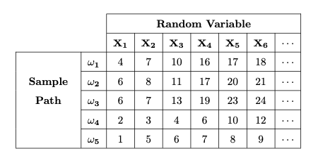
For $\omega_1$, we rolled $4,3,3,6,1,1,\ldots$ successively.

Using the stochastic process of Example 8.1.2, what is $P(X_1=1, X_4=4)$?

Using the stochastic process of Example 8.1.2, what is $P(X_t= 3 \text{ for some } t\in T)$?

Using the stochastic process of Example 8.1.2, what is $P(X_t \neq 10 \text{ for all } t\in T)$?

These are all examples of questions that we will learn to answer.

What should also be noted in Example 8.1.2 is that in performing the underlying experiment to observe $X_2$, we necessarily observe $X_1$ (before we can roll the die twice, we have to roll it once). Therefore it could be argued that it makes more natural sense to study $\rho_{X_1}$ and $\rho_{X_2 \mid X_1}$, rather than $\rho_{X_1}$ and $\rho_{X_2}$. This argument is true more generally since the parameter set $T$ typically has a time-related or sequential interpretation: we can study $\rho_{X_1}, \rho_{X_2 \mid X_1}, \rho_{X_3 \mid X_1, X_2}, \ldots \rho_{X_{n+1} \mid X_1, X_2, \ldots ,X_n}$.

This highlights a key feature of stochastic processes: the transitions from one state to another state.

8.2 Defintion of Markov Chains

A Markov Chain is a type of stochastic processes.

A stochastic process $\{ X_t: t \geq 0 \}$ is a Markov chain if $$P \left( X_{t+1} = x_{t+1} \mid X_{0} = x_{0}, \ldots, X_{t} = x_{t} \right) = P \left( X_{t+1} = x_{t+1} \mid X_{t} = x_{t} \right).$$ for all $t \geq 0$ and states $x_0, x_1, \ldots, x_n, x_{n+1}$.

This is to say, that when trying to predict the future state of a Markov chain it is only important to know the present state and not how the process arrived at this state.

The stochastic processes in Example 8.1.2 and Example 8.1.3 were Markov Chains.

Set $X_0 = X_1=1$. To define $X_t$ for $t \geq 2$, one tosses a coin. If a head is obtained then set $X_t = X_{t-1} + X_{t-2}$, and if a tails is obtained set $X_t=0$. Explain why $\left\{ X_t : t \geq 0 \right\}$ is not a Markov chain.

In the event of tossing a head clearly $X_t$ is dependent on both the value of $X_{t-1}$ and $X_{t-2}$, not just the current state $X_{t-1}$. This is in contradiction to Definition 8.2.1 of a Markov chain.

Identifying Markov chains within your workplace is a key skill for DATA2002. Many Markov chains will have a great number of states.

A Markov chain $\left\{ X_t: t \geq 0 \right\}$ is called time-homogeneous if $$P(X_{t+1} =j \mid X_t =i) = P(X_{1} =j \mid X_0 =i)$$ for all $t \geq 0$ and for all $i,j \in S$.

Informally time-homogeneouity means that the probabilities regarding transitions between states do not change with time. In this module, we only consider time-homogeneous Markov chains.

Clearly Example 8.1.3 is a time-homogeneous Markov chain.

Consider a time-homogeneous Markov chain $\left\{ X_t: t \geq 0 \right\}$. The transition probabilities are the values $$p_{ij} = P(X_{1} =j \mid X_0 =i).$$

8.3 Transition Matrix

The transition probabilities introduced in Definition 8.2.4 play a key role in the analysis of Markov chains. As an efficient storing technique we introduce the transition probability matrix.

The $\lvert S \rvert \times \lvert S \rvert$ matrix $P = (p_{ij})$, where the entry in the $i^{th}$ row and $j^{th}$ column is the transition probability $p_{i,j}$, is called the transition probability matrix.

Note that any transition probability matrix $P = (p_{ij})$:

• $p_{ij} \geq 0$ for all $i,j \in S$, or equivalently every matrix entry is non-negative;

• $\sum\limits_{j \in S} p_{ij} = 1$ for all $i \in S$, or equivalently the entries in each row of the matrix sum to $1$.

Any matrix that satisfies both of these conditions is called a stochastic matrix.

What is the transition probability matrix $P$ of the stochastic process in Example 8.1.3?

Allowing the index 1 to correspond to Latte Da and index 2 correspond to Deja Brew, from the description of the problem we have $$\begin{align*} p_{11} &= P \big( X_{t+1} = \text{Latte Da} = 1 \mid X_{t} = \text{Latte Da} = 1 \big) = \frac{1}{6}, \\[5pt] p_{12} &= P \big( X_{t+1} = \text{Deja Brew} = 2 \mid X_{t} = \text{Latte Da} = 1 \big) = \frac{5}{6}, \\[5pt] p_{21} &= P \big( X_{t+1} = \text{Latte Da} = 1 \mid X_{t} = \text{Deja Brew} = 2 \big) = \frac{1}{3}, \\[5pt] p_{22} &= P \big( X_{t+1} = \text{Deja Brew} = 2 \mid X_{t} = \text{Deja Brew} = 2 \big) = \frac{2}{3}. \end{align*}$$

Therefore the transition probability matrix is given by $$P = \begin{pmatrix} \frac{1}{6} & \frac{5}{6} \\ \frac{1}{3} & \frac{2}{3} \end{pmatrix}.$$

What is the transition probability matrix $P$ of the stochastic process in Example 8.1.2?

Suppose that $X_t = n$ for some positive integer $n$. Then since the fair die has an equal chance of rolling each of $1,2,3,4,5,6$ there is a $\frac{1}{6}$ chance that $X_{t+1}$ is equal to each of $n+1$, $n+2$, $n+3$, $n+4$, $n+5$, $n+6$. Specifically $$\begin{align*} p_{n,n+1} &= P \big( X_{t+1} = n+1 \mid X_{t} = n \big) = \frac{1}{6}, \\[5pt] p_{n,n+2} &= P \big( X_{t+1} = n+2 \mid X_{t} = n \big) = \frac{1}{6}, \\[5pt] p_{n,n+3} &= P \big( X_{t+1} = n+3 \mid X_{t} = n \big) = \frac{1}{6}, \\[5pt] p_{n,n+4} &= P \big( X_{t+1} = n+4 \mid X_{t} = n \big) = \frac{1}{6}, \\[5pt] p_{n,n+5} &= P \big( X_{t+1} = n+5 \mid X_{t} = n \big) = \frac{1}{6}, \\[5pt] p_{n,n+6} &= P \big( X_{t+1} = n+6 \mid X_{t} = n \big) = \frac{1}{6}, \\[5pt] p_{n,j} &= P \big( X_{t+1} = j \mid X_{t} = n \big) = 0, \end{align*}$$ where $j \neq n+1,n+2,n+3,n+4,n+5,n+6$. Therefore the transition probability matrix is given by $$P = \begin{pmatrix} 0 & \frac{1}{6} & \frac{1}{6} & \frac{1}{6} & \frac{1}{6} & \frac{1}{6} & \frac{1}{6} & 0 & 0 & 0 & 0 & 0 & \cdots \\ 0 & 0 & \frac{1}{6} & \frac{1}{6} & \frac{1}{6} & \frac{1}{6} & \frac{1}{6} & \frac{1}{6} & 0 & 0 & 0 & 0 & \cdots \\ 0 & 0 & 0 & \frac{1}{6} & \frac{1}{6} & \frac{1}{6} & \frac{1}{6} & \frac{1}{6} & \frac{1}{6} & 0 & 0 & 0 & \cdots \\ 0 & 0 & 0 & 0 & \frac{1}{6} & \frac{1}{6} & \frac{1}{6} & \frac{1}{6} & \frac{1}{6} & \frac{1}{6} & 0 & 0 & \cdots \\ 0 & 0 & 0 & 0 & 0 & \frac{1}{6} & \frac{1}{6} & \frac{1}{6} & \frac{1}{6} & \frac{1}{6} & \frac{1}{6} & 0 & \cdots \\ 0 & 0 & 0 & 0 & 0 & 0 & \frac{1}{6} & \frac{1}{6} & \frac{1}{6} & \frac{1}{6} & \frac{1}{6} & \frac{1}{6} & \cdots \\ 0 & 0 & 0 & 0 & 0 & 0 & 0 & \frac{1}{6} & \frac{1}{6} & \frac{1}{6} & \frac{1}{6} & \frac{1}{6} & \cdots \\ 0 & 0 & 0 & 0 & 0 & 0 & 0 & 0 & \frac{1}{6} & \frac{1}{6} & \frac{1}{6} & \frac{1}{6} & \cdots \\ 0 & 0 & 0 & 0 & 0 & 0 & 0 & 0 & 0 & \frac{1}{6} & \frac{1}{6} & \frac{1}{6} & \cdots \\ 0 & 0 & 0 & 0 & 0 & 0 & 0 & 0 & 0 & 0 & \frac{1}{6} & \frac{1}{6} & \cdots \\ \vdots & \vdots & \vdots & \vdots & \vdots & \vdots & \vdots & \vdots & \vdots & \vdots & \vdots & \vdots & \ddots \\ \end{pmatrix}.$$

This notion of transition probabilities can extended from one-step transitions to $n$-step transitions. Specifically set $$p_{ij}^{(n)} = P \big( X_{n}=j \mid X_0 =i \big).$$ Note that due to the Markov chains we are considering being time-homogeneous, we have $$P \big( X_{n}=j \mid X_0 =i \big) = P\big( X_{t+n}=j \mid X_t =i \big).$$ This is to say, only the number of steps between our known state and the future event we wish to find the probability of matters, not the time at which this is happening.

The $\lvert S \rvert \times \lvert S \rvert$ matrix $P^{(n)} = \left(p_{ij}^{(n)} \right)$, where the entry in the $i^{th}$ row and $j^{th}$ column is the $n$-step transition probability $p_{ij}^{(n)}$, is called the n-step transition probability matrix.

What is the $2$-step transition probability matrix $P^{(2)}$ of the stochastic process in Example 8.1.3.

Again allowing the index 1 to correspond to Latte Da and index 2 correspond to Deja Brew, from the description of the problem we can calculate $$\begin{align*} p_{11}^{(2)} &= P \big( X_{t+2}=1 \mid X_t =1 \big) \\[3pt] &= P \big( X_{t+2}=1, X_{t+1}=1 \mid X_t =1 \big) + \big( X_{t+2}=1, X_{t+1}=2 \mid X_t =1 \big) \\[3pt] &= \frac{1}{6} \cdot \frac{1}{6} + \frac{5}{6} \cdot \frac{1}{3} \\[3pt] &= \frac{11}{36}, \\[9pt] p_{12}^{(2)} &= P \big( X_{t+2}=2 \mid X_t =1 \big) \\[3pt] &= P \big( X_{t+2}=2, X_{t+1}=1 \mid X_t =1 \big) + \big( X_{t+2}=2, X_{t+1}=2 \mid X_t =1 \big) \\[3pt] &= \frac{1}{6} \cdot \frac{5}{6} + \frac{5}{6} \cdot \frac{2}{3} \\[3pt] &= \frac{25}{36}, \\[9pt] p_{21}^{(2)} &= P \big( X_{t+2}=1 \mid X_t =2 \big) \\[3pt] &= P \big( X_{t+2}=1, X_{t+1}=1 \mid X_t =2 \big) + \big( X_{t+2}=1, X_{t+1}=2 \mid X_t =2 \big) \\[3pt] &= \frac{1}{3} \cdot \frac{1}{6} + \frac{2}{3} \cdot \frac{1}{3} \\[3pt] &= \frac{5}{18}, \\[9pt] p_{22}^{(2)} &= P \big( X_{t+2}=2 \mid X_t =2 \big) \\[3pt] &= P \big( X_{t+2}=2, X_{t+1}=1 \mid X_t =2 \big) + \big( X_{t+2}=2, X_{t+1}=2 \mid X_t =2 \big) \\[3pt] &= \frac{1}{3} \cdot \frac{5}{6} + \frac{2}{3} \cdot \frac{2}{3} \\[3pt] &= \frac{13}{18}. \end{align*}$$

Therefore the $2$-step transition probability matrix is given by $$P^{(2)} = \begin{pmatrix} \frac{11}{36} & \frac{25}{36} \\ \frac{5}{18} & \frac{13}{18} \end{pmatrix}.$$

The following theorem gives us an easy way to calculate $n$-step transition probability matrix.

Chapman-Kolmogorov Equations: The transition probability matrix $P$ and the $n$-step transition probability matrix $P^{(n)}$ satisfy the equation $$P^{(n)} = P^n.$$

What is the $2$-step transition probability matrix $P^{(2)}$ of the stochastic process in Example 8.1.2.

By the Chapman-Kolmogorov equations, the question is equivalent to calculating $P^2$ where $P$ is the transition probability matrix calculated in Example 8.3.3. Specifically $$\begin{align*} P^{(2)} &= P^2 \\[9pt] &= \begin{pmatrix} 0 & \frac{1}{6} & \frac{1}{6} & \frac{1}{6} & \frac{1}{6} & \frac{1}{6} & \frac{1}{6} & 0 & 0 & 0 & 0 & 0 & \cdots \\ 0 & 0 & \frac{1}{6} & \frac{1}{6} & \frac{1}{6} & \frac{1}{6} & \frac{1}{6} & \frac{1}{6} & 0 & 0 & 0 & 0 & \cdots \\ 0 & 0 & 0 & \frac{1}{6} & \frac{1}{6} & \frac{1}{6} & \frac{1}{6} & \frac{1}{6} & \frac{1}{6} & 0 & 0 & 0 & \cdots \\ 0 & 0 & 0 & 0 & \frac{1}{6} & \frac{1}{6} & \frac{1}{6} & \frac{1}{6} & \frac{1}{6} & \frac{1}{6} & 0 & 0 & \cdots \\ 0 & 0 & 0 & 0 & 0 & \frac{1}{6} & \frac{1}{6} & \frac{1}{6} & \frac{1}{6} & \frac{1}{6} & \frac{1}{6} & 0 & \cdots \\ 0 & 0 & 0 & 0 & 0 & 0 & \frac{1}{6} & \frac{1}{6} & \frac{1}{6} & \frac{1}{6} & \frac{1}{6} & \frac{1}{6} & \cdots \\ 0 & 0 & 0 & 0 & 0 & 0 & 0 & \frac{1}{6} & \frac{1}{6} & \frac{1}{6} & \frac{1}{6} & \frac{1}{6} & \cdots \\ 0 & 0 & 0 & 0 & 0 & 0 & 0 & 0 & \frac{1}{6} & \frac{1}{6} & \frac{1}{6} & \frac{1}{6} & \cdots \\ 0 & 0 & 0 & 0 & 0 & 0 & 0 & 0 & 0 & \frac{1}{6} & \frac{1}{6} & \frac{1}{6} & \cdots \\ 0 & 0 & 0 & 0 & 0 & 0 & 0 & 0 & 0 & 0 & \frac{1}{6} & \frac{1}{6} & \cdots \\ \vdots & \vdots & \vdots & \vdots & \vdots & \vdots & \vdots & \vdots & \vdots & \vdots & \vdots & \vdots & \ddots \\ \end{pmatrix}^2 \\[9pt] &= \begin{pmatrix} 0 & 0 & \frac{1}{36} & \frac{1}{18} & \frac{1}{12} & \frac{1}{9} & \frac{5}{36} & \frac{1}{6} & \frac{5}{36} & \frac{1}{9} & \frac{1}{12} & \frac{1}{18} & \frac{1}{36} & 0 & 0 & \cdots \\ 0 & 0 & 0 & \frac{1}{36} & \frac{1}{18} & \frac{1}{12} & \frac{1}{9} & \frac{5}{36} & \frac{1}{6} & \frac{5}{36} & \frac{1}{9} & \frac{1}{12} & \frac{1}{18} & \frac{1}{36} & 0 & \cdots \\ 0 & 0 & 0 & 0 & \frac{1}{36} & \frac{1}{18} & \frac{1}{12} & \frac{1}{9} & \frac{5}{36} & \frac{1}{6} & \frac{5}{36} & \frac{1}{9} & \frac{1}{12} & \frac{1}{18} & \frac{1}{36} & \cdots \\ 0 & 0 & 0 & 0 & 0 & \frac{1}{36} & \frac{1}{18} & \frac{1}{12} & \frac{1}{9} & \frac{5}{36} & \frac{1}{6} & \frac{5}{36} & \frac{1}{9} & \frac{1}{12} & \frac{1}{18} & \cdots \\ 0 & 0 & 0 & 0 & 0 & 0 & \frac{1}{36} & \frac{1}{18} & \frac{1}{12} & \frac{1}{9} & \frac{5}{36} & \frac{1}{6} & \frac{5}{36} & \frac{1}{9} & \frac{1}{12} & \cdots \\ 0 & 0 & 0 & 0 & 0 & 0 & 0 & \frac{1}{36} & \frac{1}{18} & \frac{1}{12} & \frac{1}{9} & \frac{5}{36} & \frac{1}{6} & \frac{5}{36} & \frac{1}{9} & \cdots \\ 0 & 0 & 0 & 0 & 0 & 0 & 0 & 0 & \frac{1}{36} & \frac{1}{18} & \frac{1}{12} & \frac{1}{9} & \frac{5}{36} & \frac{1}{6} & \frac{5}{36} & \cdots \\ 0 & 0 & 0 & 0 & 0 & 0 & 0 & 0 & 0 & \frac{1}{36} & \frac{1}{18} & \frac{1}{12} & \frac{1}{9} & \frac{5}{36} & \frac{1}{6} & \cdots \\ 0 & 0 & 0 & 0 & 0 & 0 & 0 & 0 & 0 & 0 & \frac{1}{36} & \frac{1}{18} & \frac{1}{12} & \frac{1}{9} & \frac{5}{36} & \cdots \\ 0 & 0 & 0 & 0 & 0 & 0 & 0 & 0 & 0 & 0 & 0 & \frac{1}{36} & \frac{1}{18} & \frac{1}{12} & \frac{1}{9} & \cdots \\ \vdots & \vdots & \vdots & \vdots & \vdots & \vdots & \vdots & \vdots & \vdots & \vdots & \vdots & \vdots & \vdots & \vdots & \vdots & \ddots \\ \end{pmatrix} \end{align*}$$

What is the $n$-step transition probability matrix $P^{(n)}$ of the stochastic process in Example 8.1.3.

By the Chapman-Kolmogorov equations, the question is equivalent to calculating $P^n$ where $P$ is the transition probability matrix calculated in Example 8.3.2. Specifically $$P^{(n)} = P^n = \begin{pmatrix} \frac{1}{6} & \frac{5}{6} \\ \frac{1}{3} & \frac{2}{3} \end{pmatrix}^n.$$

To calculate this high order of $P$, we first diagonalise: recall from Mathematics for Data Science that $P=MDM^{-1}$ where $D$ is the diagonal matrix of eigenvalues of $P$, and $M$ is the matrix whose $i^{th}$ column is the eigenvector of $P$ corresponding to the $i^{th}$ eigenvalue in $D$. For $P$, we can check that $$D = \begin{pmatrix} 1 & 0 \\ 0 & -\frac{1}{6} \end{pmatrix} \qquad \text{and} \qquad M=\begin{pmatrix} 1 & 5 \\ 1&-2 \end{pmatrix}.$$ It follows that $$\begin{align*} P^{(n)} &= P^n \\[9pt] &= (MDM^{-1}) (MDM^{-1}) \ldots (MDM^{-1}) \\[9pt] &= M D^n M^{-1} \\[9pt] &= \begin{pmatrix} 1 & 5 \\ 1 & -2 \end{pmatrix} \begin{pmatrix} 1 & 0 \\ 0 & -\frac{1}{6} \end{pmatrix}^n \begin{pmatrix} \frac{2}{7} & \frac{5}{7} \\ \frac{1}{7} & -\frac{1}{7} \end{pmatrix} \\[9pt] &= \begin{pmatrix} 1 & 5 \\ 1 & -2 \end{pmatrix} \begin{pmatrix} 1 & 0 \\ 0 & \left(-\frac{1}{6} \right)^n \end{pmatrix} \begin{pmatrix} \frac{2}{7} & \frac{5}{7} \\ \frac{1}{7} & -\frac{1}{7} \end{pmatrix} \\[9pt] &= \begin{pmatrix} 1 & 5\left(-\frac{1}{6} \right)^n \\ 1 & -2\left(-\frac{1}{6} \right)^n \end{pmatrix} \begin{pmatrix} \frac{2}{7} & \frac{5}{7} \\ \frac{1}{7} & -\frac{1}{7} \end{pmatrix} \\[9pt] &= \begin{pmatrix} \frac{2}{7} + \frac{5}{7} \left(-\frac{1}{6} \right)^n & \frac{5}{7} - \frac{5}{7} \left(-\frac{1}{6} \right)^n \\ \frac{2}{7} - \frac{2}{7} \left(-\frac{1}{6} \right)^n & \frac{5}{7} + \frac{2}{7} \left(-\frac{1}{6} \right)^n \end{pmatrix} \end{align*}$$

Approximate the probability that Mary Berry goes to Deja Brew on some trip infinitely far in the future.

8.4 Hitting Probabilities and Hitting Times

Given a Markov chain and a current state, one can ask about the probabilities of ever achieving other states.

Given two distinct states $i,j$ of a Markov chain, the hitting probability denoted $f_{ij}$ is the probability of ever reaching state $j$ in the future given that the current state is $i$. Mathematically $$f_{ij} = P \big( X_t = j \text{ for some } t\geq 1 \mid X_0 =i \big).$$

Often the best way to calculate $f_{ij}$, is to split the possible sample path into cases based on the first step. Specifically $$P \big( X_t = j \text{ for some } t\geq 1 \mid X_0 =i \big) = \sum\limits_{k \in S} P \big( X_t = j \text{ for some } t\geq 1, \text{ and } X_1=k \mid X_0 =i \big).$$ This right hand side of this equation can then be conditioned using the general probability identity $P \left( A \cap B \right) = P(A \mid B) P(B)$. This is fully illustrated by the following example:

A company has a new website which consists of 4 pages: a Front Page which links to all other pages, an About Us page and a Contact Us page which both link to each other and back to the front page, and an Our Staff page which has no links on it. A prospective customer starts at a random page, and chooses from the available links on the page with equal probability to decide which the next page is. At all future times they repeat this procedure. Thinking of the above process as a Markov chain, and in doing so labeling the pages as $1,2,3,4$ according to the order they are listed above, calculate the hitting times $f_{12}$, $f_{13}$, $f_{23}$, $f_{32}$.

The Markov chain can be described diagrammatically:

The transition matrix is therefore $$P = \begin{pmatrix} 0 & \frac{1}{3} & \frac{1}{3} & \frac{1}{3} \\ \frac{1}{2} & 0 & \frac{1}{2} & 0 \\ \frac{1}{2} & \frac{1}{2} & 0 & 0 \\ 0 & 0 & 0 & 1 \end{pmatrix}.$$

Calculating the hitting probability using the recommended method: $$\begin{align*} f_{12} &= P \left( X_n = 2 \text{ for some } n\geq 1 \mid X_0 =1 \right) \\[5pt] &= \sum\limits_{k=1}^{4} P \left( X_n = 2 \text{ for some } n\geq 1, \text{ and } X_1 =k \mid X_0 =1 \right) \\[5pt] &= \sum\limits_{k=1}^{4} P \left( X_n = 2 \text{ for some } n\geq 1 \mid X_1 =k, X_0 =1 \right) \cdot P \left( X_1=k \mid X_0=1 \right) \\[5pt] &= \sum\limits_{k=1}^{4} P \left( X_n = 2 \text{ for some } n\geq 1 \mid X_1 =k \right) \cdot p_{1k} \\[5pt] &= P \left( X_n = 2 \text{ for some } n\geq 1 \mid X_1 =1 \right) \cdot p_{11} \\ &\hspace{50pt} + P \left( X_n = 2 \text{ for some } n\geq 1 \mid X_1 =2 \right) \cdot p_{12} \\ &\hspace{100pt}+ P \left( X_n = 2 \text{ for some } n\geq 1 \mid X_1 =3 \right) \cdot p_{13} \\ &\hspace{150pt} + P \left( X_n = 2 \text{ for some } n\geq 1 \mid X_1 =4 \right) \cdot p_{14} \\[5pt] &= f_{12}\cdot p_{11} + 1 \cdot p_{12} + f_{32} \cdot p_{13} + f_{42} \cdot p_{14} \\[5pt] &= f_{12}\cdot 0 + 1 \cdot \frac{1}{3} + f_{32} \cdot \frac{1}{3} + 0 \cdot \frac{1}{3} \\[5pt] &= \frac{1}{3} + \frac{1}{3} f_{32}. \hspace{100pt} (*) \end{align*}$$

So we have an expression for $f_{12}$ in terms of $f_{32}$. Let’s calculate $f_{32}$: $$\begin{align*} f_{32} &= P \left( X_n = 2 \text{ for some } n\geq 1 \mid X_0 =3 \right) \\[5pt] &= \sum\limits_{k=1}^{4} P \left( X_n = 2 \text{ for some } n\geq 1, \text{ and } X_1 =k \mid X_0 =3 \right) \\[5pt] &= \sum\limits_{k=1}^{4} P \left( X_n = 2 \text{ for some } n\geq 1 \mid X_1 =k, X_0 =3 \right) \cdot P \left( X_1=k \mid X_0=3 \right) \\[5pt] &= \sum\limits_{k=1}^{4} P \left( X_n = 2 \text{ for some } n\geq 1 \mid X_1 =k \right) \cdot p_{3k} \\[5pt] &= P \left( X_n = 2 \text{ for some } n\geq 1 \mid X_1 =1 \right) \cdot p_{31} \\ &\hspace{50pt} + P \left( X_n = 2 \text{ for some } n\geq 1 \mid X_1 =2 \right) \cdot p_{32} \\ &\hspace{100pt}+ P \left( X_n = 2 \text{ for some } n\geq 1 \mid X_1 =3 \right) \cdot p_{33} \\ &\hspace{150pt} + P \left( X_n = 2 \text{ for some } n\geq 1 \mid X_1 =4 \right) \cdot p_{34} \\[5pt] &= f_{12}\cdot p_{31} + 1 \cdot p_{32} + f_{32} \cdot p_{33} + f_{42} \cdot p_{34} \\[5pt] &= f_{12}\cdot \frac{1}{2} + 1 \cdot \frac{1}{2} + f_{32} \cdot 0 + 0 \cdot 0 \\[5pt] &= \frac{1}{2} + \frac{1}{2} f_{12}. \hspace{100pt} (**) \end{align*}$$

Substituting equation $(**)$ into equation $(*)$: $$f_{12} = \frac{1}{3} + \frac{1}{3} f_{32} =\frac{1}{3} + \frac{1}{3} \left( \frac{1}{2} + \frac{1}{2} f_{12} \right) = \frac{1}{3} + \frac{1}{6} + \frac{1}{6} f_{12}$$ $$\frac{5}{6} f_{12} = \frac{1}{2}$$ $$f_{12} = \frac{3}{5}.$$ Therefore $$f_{32} = \frac{1}{2} + \frac{1}{2} f_{12} = \frac{1}{2} + \frac{1}{2} \cdot \frac{3}{5} = \frac{4}{5}.$$ By the symmetry of the structure of the website with regards to the pages About Us and Contact Us pages, we have $$f_{13} = \frac{3}{5} \qquad \text{and} \qquad f_{23}=\frac{4}{5}.$$

As a side note to Example 8.4.2, note that once one gets on the Our staff page that there is no hyperlink away from this page. Therefore $f_{4,1} = f_{4,2} = f_{4,3} = 0$.

Calculate $f_{14}$, $f_{24}$ and $f_{34}$ in Example 8.4.2.

Hitting time probabilities can be decomposed into a sum of probabilities such a transition takes place in exactly $n$ steps.

Given two distinct states $i,j$ of a Markov chain, define $f_{ij}^{(n)}$ to be the probability of reaching state $j$ for the first time in exactly $n$ steps given that the current state is $i$. Mathematically $$f_{ij}^{(n)} = P \big( X_1 \neq j, X_2 \neq j, \ldots, X_{n-1} \neq j, X_n = j \mid X_0 =i \big).$$

What is the difference between $f_{ij}^{(n)}$ and $p_{ij}^{(n)}$?

Defintion 8.4.1 and Defintion 8.4.3 collectively lead to the identity $$f_{ij} = \sum\limits_{n\geq 1} f_{ij}^{(n)}.$$

Consider again the company website from Example 8.4.2. Starting on the Front Page, I begin to browse the website by clicking on hyperlinks. What is the probability that I return to the Front Page for the first time after $n$ movements, where $n \geq 1$.

Mathematically the question is asking us to calculate $f_{11}^{(n)}$. To do so, we will look at all paths starting at state $1$ which first return to state $1$ after $n$ time steps. Since there is no link to leave the Our Staff page, that is there is no way for the Markov chain to leave state $4$, such a path will not visit this page of the website. Furthermore the path only visits state $1$, the Front Page, at the beginning and end, all other intermediary states will necessarily fluctuate between states $2$ and $3$.

Calculate $$\begin{align*} f_{11}^{(1)} &= P \left( X_1=1 \mid X_0=1 \right) \\[3pt] &= 0, \\[9pt] f_{11}^{(2)} &= P \left( X_1 \neq 1, X_2 =1 \mid X_0=1 \right) \\[3pt] &= P \left( X_1=2, X_2=1 \mid X_0 =1 \right) + P \left( X_1=3, X_2=1 \mid X_0 =1 \right) \\[3pt] &= P \left( X_1=2 \mid X_0 =1 \right) \cdot P \left( X_2=1 \mid X_1 =2 \right) + P \left( X_1=3 \mid X_0 =1 \right) \cdot P \left( X_2=1 \mid X_1 =3 \right) \\[3pt] &= \frac{1}{3} \cdot \frac{1}{2} + \frac{1}{3} \cdot \frac{1}{2} \\[3pt] &= \frac{1}{3} \\[9pt] f_{11}^{(3)} &= P \left( X_1, X_2 \neq 1, X_3 =1 \mid X_0=1 \right) \\[3pt] &= P \left( X_1=2, X_2=3, X_3=1 \mid X_0 =1 \right) + P \left( X_1=3, X_2=2, X_3 =1 \mid X_0 =1 \right) \\[3pt] &= P \left( X_1=2 \mid X_0 =1 \right) \cdot P \left( X_2=3 \mid X_1 =2 \right) \cdot P \left( X_3=1 \mid X_2 =3 \right) \\ &\hspace{50pt} + P \left( X_1=3 \mid X_0 =1 \right) \cdot P \left( X_2=2 \mid X_1 =3 \right) \cdot P \left( X_3=1 \mid X_2 =2 \right) \\[3pt] &= \frac{1}{3} \cdot \frac{1}{2} \cdot \frac{1}{2} + \frac{1}{3} \cdot \frac{1}{2} \cdot \frac{1}{2} \\[3pt] &= \frac{1}{6} \\[9pt] & \vdots \\[9pt] f_{11}^{(n)} &= P \left( X_1, X_2, \ldots , X_{n-1} \neq 1, X_n =1 \mid X_0=1 \right) \\[3pt] &= P \left( X_1 =2, X_2=3, \ldots , X_n =1 \mid X_0=1 \right) + P \left( X_1 =3, X_2=2, \ldots , X_n =1 \mid X_0=1 \right) \\[3pt] &= \frac{1}{3} \cdot \frac{1}{2^{n-1}} + \frac{1}{3} \cdot \frac{1}{2^{n-1}} \\[3pt] &= \frac{1}{3} \cdot \frac{1}{2^{n-2}} \\[9pt] & \vdots \end{align*}$$

The concept of $n$-step hitting times $f_{ij}^{(n)}$ leads to consideration of the random variable $T_{i}^{j}$, defined formally below, which governs when the process first hits the state $j$ starting from state $i$.

The hitting time, denoted $T_{i}^{j}$, is the random variable which returns the quantity $$T_i^j = \inf \left\{ n>0 : X_n = j \text{ given } X_0=i \right\}$$ for a randomly chosen sample path of the Markov chain.

If we never reach state $j$ from state $i$ in the sample path then $T_i^j = \infty$.

Note that $$f_{ij}^{(n)} = P \left( T_i^j = n \right).$$

Consider again the Markov chain of Example 8.4.2 based on traversing a companys’ website. Calculate $P \left( T_1^2 = 1\right), P \left( T_1^2 = 2\right), P \left( T_1^2 = 3\right)$.

We calculate $$\begin{align*} P \left( T_1^2 = 1 \right) &= f_{12}^{(1)} \\[3pt] &= p_{12} \\[3pt] &= \frac{1}{3}, \\[9pt] P \left( T_1^2 = 2 \right) &= f_{12}^{(2)} \\[3pt] &= P \left( X_1=1, X_2=2 \mid X_0=1 \right) + P \left( X_1=3, X_2=2 \mid X_0=1 \right) \\ & \hspace{100pt}+ P \left( X_1=4, X_2=2 \mid X_0=1 \right) \\[3pt] &= p_{11}\cdot p_{12} + p_{13}\cdot p_{32} + p_{14}\cdot p_{42}, \\[3pt] &= 0 \cdot \frac{1}{3} + \frac{1}{3} \cdot \frac{1}{2} + \frac{1}{3} \cdot 0 \\[3pt] &= \frac{1}{6}, \\[9pt] P \left( T_1^2 = 3 \right) &= f_{12}^{(3)} \\[3pt] &= p_{11}\cdot f_{12}^{(2)} + p_{13}\cdot f_{32}^{(2)} + p_{14}\cdot f_{42}^{(2)}, \\[3pt] &= 0\cdot f_{12}^{(2)} + \frac{1}{3} \cdot f_{32}^{(2)} + \frac{1}{3} \cdot 0, \\[3pt] &= \frac{1}{3} f_{32}^{(2)}, \\[3pt] &= \frac{1}{3} (p_{31} \cdot p_{12}) \\[3pt] &= \frac{1}{3} \cdot \frac{1}{2} \cdot \frac{1}{3} \\[3pt] &= \frac{1}{18} \end{align*}$$

In the calculation of $P(T_1^2 =2)$ why did we ignore the path where $X_0=1, X_1=2, X_2=2$.

Renewal Equation: Given a Markov chain with $n$-step transition probabilities $p_{ij}^{(n)}$, and hitting probabilities $f_{ij}$, one has $$p_{ij}^{(n)} = \sum\limits_{k=1}^{n} f_{ij}^{(k)} p_{jj}^{(n-k)}.$$

Informally the renewal equation states that the probability of going from state $i$ to state $j$ over $n$ steps can be conditioned on when we first visit state $j$.