Chapter 9 States, Recurrence and Periodicity
Suppose we have a Markov chain which is currently in state \(i\). It is natural to ask questions such as the following:
Are there any states that we cannot ever get to?
Once we leave state \(i\) are we guaranteed to get back?
If we are certain to return to \(i\) how long does this take on average?
If it is possible to return to \(i\), for what values of \(n\) is it possible to return in \(n\) steps?
To answer these questions, we study properties of a Markov chain, and it particular introduce classes of states.
9.1 Communication of States
In this section, we formalise the notion of one state being accessible from another.
A state \(i\) is said to communicate with a state \(j\) if there is a non-zero probability that a Markov chain currently in state \(i\) will move to state \(j\) in the future. Mathematically \(p_{ij}^{(n)}>0\) for some \(n \geq 0\). This is denoted by \(i \rightarrow j\).
That is to say, state \(i\) can communicate with state \(j\) if it is possible to move from \(i\) to \(j\).
Note in Defintion 9.1.1 that \(n=0\) is permitted. It follows that any state \(i\) is said communicate with itself: \(i \rightarrow i\) necessarily.

Note that if \(X_t=2\) for some \(t\), that is the Markov chain is in state 2, then one can move to state 4 for example by the path \(X_t=2, X_{t+1} = 1, X_{t+2}=4\) (other routes are available). Therefore \(2 \rightarrow 4\). Similarly \(1 \rightarrow 4\) and \(3 \rightarrow 4\).
However since \(p_{44}=1\), or equivalently \(p_{41}=p_{42}=p_{43}=0\), it is impossible for the Markov chain to leave state 4. That is state \(4\) cannot communicate with any of the states \(1,2,3\).
States \(i\) and \(j\) are said to intercommunicate if \(i \rightarrow j\) and \(j \rightarrow i\). This is denoted by \(i \leftrightarrow j\)
Considering again the Markov Chain governing the company website of Example 8.4.2, seen in Example 9.1.2, one can easily observe that \(1 \leftrightarrow 2, 2 \leftrightarrow 3\) and \(1 \leftrightarrow 3\).
However since state \(4\) does not communicate with states \(1,2\) or \(3\), it follows that state \(4\) does not intercommunicate with any of the states \(1,2\) or \(3\)
We have introduced the notions of communication and intercommunication, as we anticipate that properties of states will be shared by those that intercommunicate with each other. In this vein, one could group together all states that can intercommunicate to partition the Markov chain into communicating classes.
We introduce two notions that capture collections of states that have strong properties regarding communication together.
A set \(C\) of states is called irreducible if \(i \leftrightarrow j\), for all \(i,j \in C\).
A Markov chain is said to be irreducible itself, if the set of all states is irreducible.
A set \(C\) of states is said to be closed if for any \(i \in C\) and \(j \notin C\), then \(p_{ij}=0\).
Once a Markov chain reaches a closed state \(C\), it will subsequently never leave \(C\).
Consider the Markov chain represented by the following:
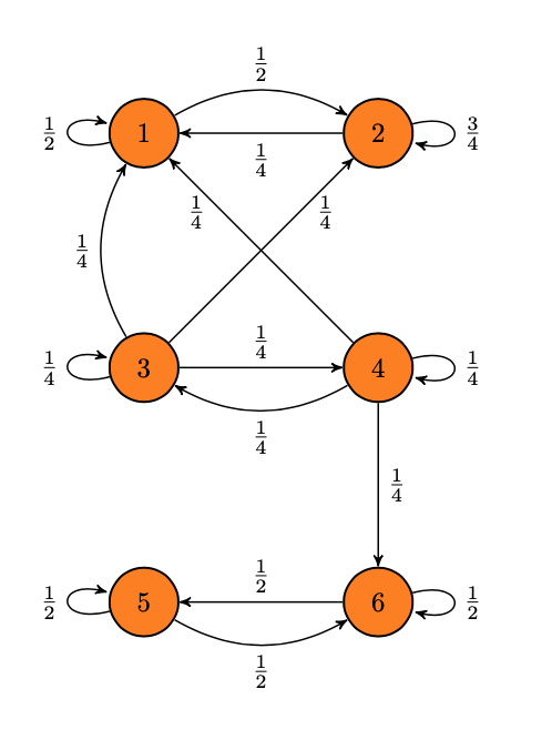
Show that the set \(\{1,2\}\) is both irreducible and closed.
From the Markov chain diagram, one can read the transition matrix for the Markov chain as
\[P = \begin{pmatrix}
\frac{1}{2} & \frac{1}{2} & 0 & 0 & 0 & 0 \\
\frac{1}{4} & \frac{3}{4} & 0 & 0 & 0 & 0 \\
\frac{1}{4} & \frac{1}{4} & \frac{1}{4} & \frac{1}{4} & 0 & 0 \\
\frac{1}{4} & 0 & \frac{1}{4} & \frac{1}{4} & 0 & \frac{1}{4} \\
0 & 0 & 0 & 0 & \frac{1}{2} & \frac{1}{2} \\
0 & 0 & 0 & 0 & \frac{1}{2} & \frac{1}{2}
\end{pmatrix}.\]
Note that \(p_{12} = \frac{1}{2}>0\) so there is a path from state \(1\) to state \(2\), and \(p_{21} = \frac{1}{4}>0\) so there is a path from state \(2\) to state \(1\). Therefore \(1 \leftrightarrow 2\), that is \(\{1,2\}\) is irreducible.
Also note \(p_{13}=p_{14}=p_{15}=p_{16}=p_{23}=p_{24}=p_{25}=p_{26}=0\), so by Definition 9.1.6 the set \(\{1,2\}\) is closed.
Therefore \(\{1,2\}\) is a closed and irreducible set.Are there any other irreducible and closed sets in the Markov chain of Example 9.1.7? What about sets that are only irreducible, and sets that are only closed?
The terminology introduced in both Defintion 9.1.5 and Definition 9.1.6 freely for the remainder of the course.
If a closed set \(C\) of states contains only one state \(i\), that is \(p_{ii} = 1\) and \(p_{ij}=0\) for all \(j \neq i\), we call \(i\) an absorbing state.
Find an absorbing state among the Markov chains we have seen in previous examples.
9.2 Recurrence
A state of a Markov chain is called recurrent if \[P[X_n = i \text{ for some } n\geq 1 \mid X_0 = i] = 1.\]
The essence of this definition is that a Markov chain that is currently in some recurrent state is certain to return to that state again in the future.
A state of a Markov chain that is not recurrent is called transient.
A Markov chain that is currently in some transient state is not certain to return to that state again in the future.
Consider the Markov Chain governing Mary Berrys’ choice of Nottingham coffee shop of Example 8.1.3, that is the Markov chain described by the diagram

Show that Latte Da is a recurrent state.
Suppose that the Mary Berry visits Latte Da on her \(t^{th}\) trip to Nottingham. Mathematically in terms of the Markov chain: \(X_t = \text{Latte Da}\). First we calculate the probability that Mary Berry doesn’t visit Latte Da on her next \(N\) visits to Nottingham.
\[\begin{align*}
&P (\text{Mary Berry doesn't visit Latte Da on next $N$ visits} \mid X_t = \text{Latte Da}) \\
=& P ( X_{t+N} = X_{t+N-1} = \cdots = X_{t+1} = \text{Deja Brew} \mid X_t = \text{Latte Da}) \\
=& P ( X_{t+N} = \text{D.B.} \mid X_{t+N-1} = \text{D.B.}) \times P ( X_{t+N-1} = \text{D.B.} \mid X_{t+N-2} = \text{D.B.}) \times \ldots \\
& \qquad \qquad \ldots \times P ( X_{t+2} = \text{D.B.} \mid X_{t+1} = \text{D.B.}) \times P ( X_{t+1} = \text{D.B.} \mid X_{t} = \text{L.D.}) \\
=& P ( X_{1} = \text{D.B.} \mid X_{0} = \text{D.B.}) \times P ( X_{1} = \text{D.B.} \mid X_{0} = \text{D.B.}) \times \ldots \\
& \qquad \qquad \ldots \times P ( X_{1} = \text{D.B.} \mid X_{0} = \text{D.B.}) \times P ( X_{1} = \text{D.B.} \mid X_{0} = \text{L.D.}) \\
&= \frac{5}{6} \times \frac{2}{3} \times \ldots \frac{2}{3} \\
&= \frac{5}{6} \left( \frac{2}{3} \right)^{N-1}
\end{align*}\]
Consider again the Markov Chain governing the company website of Example 8.4.2, seen in Example 9.1.2. Show that state 1 is a transient state.
Suppose the user is on the Home Page of the website, that is \(X_t=1\) for some \(t\). The user could click on the link to the Staff Page, that is, state 4 of the Markov chain. At this point it is impossible for the user to return to the Home Page, or state 1. That is to say, it is not certain that the Markov chain will ever return to state 1. Therefore state 1 is transiant.
If \(i \leftrightarrow j\), then state \(i\) is recurrent if and only if state \(j\) is recurrent.
It follows from Example 9.2.3 and Lemma 9.2.5 that the state Deja Brew in the Mary Berry coffee shop example is also recurrent.
Indeed Lemma 9.2.5 indicates that it makes sense to label communicating classes as either recurrent or transiant: if one state in a communicating class is recurrent/transient then all the states in that class must be recurrent/transient respectively. This leads to the following definition.
An irreducible Markov chain is said to be recurrent if it contains at least one recurrent state.
An irreducible Markov chain being recurrent as per Definition 9.2.6 is equivalent to every state of the Markov chain being recurrent.
9.3 Mean Recurrence Times
The mean recurrence time of a state \(i\), denoted \(\mu_i\), is given by \[\mu_i = \begin{cases} \sum\limits_{n \geq 1} n f_{ii}^{(n)},& \text{if state } i\text{ recurrent,} \\ \infty,& \text{if state } i \text{ transiant.} \\ \end{cases}\]
Suppose \(i\) is a recurrent state. It follows from Definition 9.3.1, that the mean recurrence time is the average time that it takes for the Markov chain currently in state \(i\) to return to \(i\). This can be seen by noting that the summation is over all possibilities for how long it could take the Markov chain to return as required, and that \(f_{ii}^{(n)}\) is the probability that the Markov chain moves from state \(i\) to state \(i\) in exactly \(n\) steps.
Calculate the mean recurrence time \(\mu_1\) for the Markov Chain governing the company website of Example 8.4.2.
Substituting in the known value of \(f_{11}^{(1)} = 0\) and \(f_{11}^{(n)} = \frac{1}{3} \cdot \frac{1}{2^{n-2}}\) where \(n \geq 2\) from Example 8.4.4 into Definition 9.3.1 obtain \[\mu_1 = \sum\limits_{n \geq 1} n f_{11}^{(n)} = f_{11}^{(1)} + \sum\limits_{n=2}^{\infty} n f_{11}^{(2)} = 0 + \sum\limits_{n=2}^{\infty} n \cdot \frac{1}{3} \cdot \frac{1}{2^{n-2}} = \frac{1}{3} \sum\limits_{n=2}^{\infty} \frac{n}{2^{n-2}}.\] Using computer code calculate \(\sum\limits_{n=2}^{\infty} \frac{n}{2^{n-2}} = 6\) and so \[\mu_1 = \frac{1}{3} \cdot 6 = 2.\]
Note that even if state \(i\) is recurrent, the mean recurrence time may still be \(\infty\).
Consider a recurrent state \(i\). The state \(i\) is said to be positive recurrent if \(\mu_i < \infty\), or null recurrent if \(\mu_i = \infty\).
It follows from Example 9.3.2 that state \(1\) in the Markov chain governing the company website is positive recurrent since \(\mu_1 =2 <\infty\).
If \(i \leftrightarrow j\), then \(i\) is positive recurrent if and only if \(j\) is positive recurrent.
This lemma provides us with a shortcut to show positive recurrence of a large number of states.
Combining Example 9.1.4, Example 9.3.4 and Lemma 9.3.5 shows that states \(2\) and state \(3\) are also positive recurrent in the running company website Markov chain example.
An irreducible Markov chain is said to be positive-recurrent if it contains at least one positive-recurrent state.
An irreducible Markov chain being positive-recurrent as per Definition 9.3.7 is equivalent to every state of the Markov chain being positive-recurrent.
Note that Lemma 9.3.5 does not tell us anything about the mean recurrent time of intercommunicating recurrent states beyond finiteness. Namely knowing that \(\mu_1 = 2\) in Example 9.3.2 does not provide any new information about \(\mu_2\) and \(\mu_3\), beyond what we would have known given \(\mu_1 < \infty\).
If a Markov chain has a finite number of states, then all recurrent states are positive.
An irreducible Markov chain with a finite number of states is positive-recurrant.
9.4 Periodicity
Consider a Markov chain in some state \(i\). Consider the values of \(n\) for which \(p_{ii}^{(n)}>0\), that is, the positive integers \(n\) for which it is possible for the Markov chain to return to \(i\) in \(n\) steps. Throughout this section we denote this collection of values by \(\{ a_1, a_2, a_3, \ldots \}\).
The period of state \(i\) is given by \[d_i = \gcd (a_1,a_2,a_3, \ldots )\]
Recall the scenario of Week 6 Questions, Questions 1 to 8:
Every year Ria chooses exactly two apprentices to compete in the fictitious competition Nottingham’s Got Mathematicians. Apprentices are recommended to Ria by Daniel and Lisa. Initially Daniel and Lisa recommend one candidate each. However if Daniel selects the apprentice who finishes second among Ria’s nominees, then this opportunity for recommendation is given to Lisa the following year. Similarly if Lisa chooses the candidate who who finishes second among Ria’s nominees, then this opportunity for recommendation is given to Daniel the following year. This rule is repeated every year, even if Daniel or Lisa choose both the candidates.
Generally Lisa is better at picking competitors: a Lisa endorsed candidate beats a Daniel endorsed candidate \(75 \%\) of the time.
This scenario can be modelled by the Markov chain:
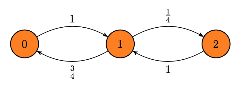
Calculate \(d_1\), the period of state \(1\).
Consider all the possible paths that start and end in state \(1\): \[\begin{align*} 1 &\rightarrow 0 \rightarrow 1 \\ 1 &\rightarrow 2 \rightarrow 1 \\ 1 &\rightarrow 0 \rightarrow 1 \rightarrow 0 \rightarrow 1 \\ 1 &\rightarrow 0 \rightarrow 1 \rightarrow 2 \rightarrow 1 \\ 1 &\rightarrow 2 \rightarrow 1 \rightarrow 0 \rightarrow 1 \\ 1 &\rightarrow 2 \rightarrow 1 \rightarrow 2 \rightarrow 1 \\ 1 &\rightarrow 0 \rightarrow 1 \rightarrow 0 \rightarrow 1 \rightarrow 0 \rightarrow 1 \\ &\vdots \end{align*}\] The lengths of these paths respectively are \(2,2,4,4,4,4,6, \ldots\). Calculate \[d_1 = \gcd ( 2,2,4,4,4,4,6, \ldots) =2.\]
This definition goes a long way towards answering the question “If it is possible to return to \(i\), for what values of \(n\) is it possible to return in \(n\) steps?” identified at the opening of the chapter. Namely for a given value \(n\), it is possible to return from to state \(i\) to state \(i\) if and only if \(d_i\) divides \(n\) exactly.
If \(i \leftrightarrow j\), then \(i\) and \(j\) have the same period: \[d_i = d_j.\]
Consider the Markov chain of Example 9.4.2. Calculate \(d_0\) and \(d_2\), the periods of states \(0\) and \(2\).
Clearly states \(0,1,2\) intercommunicate, that is, \(0 \leftrightarrow 1\) and \(1 \leftrightarrow 2\). From Example 9.4.2, we know \(d_1 = 2\) and so by Lemma 9.4.3 it follows that \(d_0=d_2=2\).
A state is said to be aperiodic if \(d_i=1\).
A Markov chain is aperiodic if all of its states are aperiodic.
Since trivially \(1\) divides all positive integers \(n\), this definition is equivalent to saying that it is possible to return to state \(i\) in any number of steps. Aperiodicity is often a feature of the most mathematically interesting Markov chains, and will be a key assumption when it comes to talking about steady states.
An absorbing state is aperiodic.