7 Chapter 7: Random Forests, Neural Nets
7.1 Current practice
Current practice in supervised machine learning roughly follows this procedure:
- Split the data into train and test sets
- We will use 70% train and 30% test. Other choices are possible.
- Use cross-validation (often 10-fold) to choose tuning parameters associated with a modeling class.
- E.g., \(\gamma\) in svm. We will limit our choices to what software provides.
- Caret package documentation lists very specific tuning parameters for each method – for the implementations supported.
- Repeat the CV approach many times (we will do it 100 times)
- Use average accuracy or other measure of fit to choose tuning parameters.
- Using CV-based tuning parameters, evaluate out of sample performance (accuracy) on the withheld test set.
7.1.1 Further rationale:
- The accuracy reported during the training phase, although it uses CV, tends to be overly optimistic.
- There is some debate about whether this is true, and it is all based on simulations, which don’t all agree.
- The withheld test data set is “pure” in some sense. It was never used in any phase of the training.
- It was never part of a fold, nor test, during the tuning parameter selection.
7.2 Feature selection
- There are several good reasons to reduce the number of features that you pass to an ML algorithm. Most do not apply with our test data, as it is small. However, with larger numbers of features:
- Reduction makes computation feasible, esp. for cross-validation steps.
- Reduction breaks correlation between features, which when left in the set, can have negative consequences (e.g., for Random Forest, the ensemble of trees will be more correlated if several variable are exchangeable due to high correlation).
- Reduction limits the curse of dimensionality, which is basically that in higher dimensions, observations are concentrated in a manner that is not conducive to many learning algorithms. Human intuition is poor, as to where the bulk of observations will be located.
- Reduction drops variables that do not improve predictive performance; some methods are more sensitive to this (wasting degrees of freedom/parameters).
- From Guyon and Elisseeff (2003) - in Readings on Brightspace: “The objective of variable selection is three-fold: improving the prediction performance of the predictors, providing faster and more cost-effective predictors, and providing a better understanding of the underlying process that generated the data.”
7.2.1 Approaches to Feature Selection (rough):
- Filter methods: some version of importance scoring applied to features
- Often based on a statistical test (think: looking at a correlation table)
- Unless they are “wrapped” into a cross-validation procedure, and even when they are, likely to lead to out of sample performance problems due to overfitting.
- Wrapper methods: The “procedure” for setting tuning parameters also explores the space of features, using heuristics (often statistical tests)
- Example: Forwards/Backwards elimination; Recursive Feature Elimination (for RF; in the caret package).
- Embedded methods: These are models that have regularization parameters built-in
- Example: lasso, which shrinks many parameters to zero, essentially eliminating variables. Advantage: can be included in the cross-validation as there is only one model, and you are just tuning it.
7.2.2 Warning when using a feature selection method:
- Feature selection should be performed on data that is not used for training or testing.
- If you have used all of the data to tweak any aspect of the model, then there is no such thing as out of sample performance
- Arguably you could do feature selection on the training set, tune using CV and then only evaluate performance on the test set. However, even the choices for the features and resulting tuning parameters are likely overfitting, reducing out of sample performance (see main point).
- Feature selection embedded (in the model) is likely to work (of course tuning with CV), but there is mixed opinion about this.
- And only methods including regularization parameters are set up this way.
- Given that feature selection has many hidden pitfalls, you might limit your use of it to:
- Substantive knowledge
- Similar to model fitting in which parameters matter, consider correlation tables of predictors (but exclude the outcome: contrary to many ML approaches) to remove “redundant” ones.
7.2.3 Setup for our examples:
- We augment the feature set in penguins data using 2-way products (interactions) and square root of measurement.
- We augment the feature set in Crabs data using two interaction terms.
- Random Forests should be able to “choose wisely” among our augmented features, so there is no downside to their inclusion
- Neural Nets should down-weight the influence of extraneous features, so they may be robust to any additional variation induced by the augmentation.
- We may find out something a bit unexpected with penguins data and Neural Nets
7.2.4 Variable importance
- One approach to assessing variable importance, based on a suggestion by Breiman, is to re-compute accuracy with a particular variable randomly shuffled and note how much accuracy drops.
- Idea: if you change a predictor to “noise” through reshuffling, then if it mattered for prediction, you should do worse.
- Fine point: what sample do you reshuffle? There are many choices, ranging from “out of the bag” (OOB) samples that come from the random forest bagging procedure, to using parts of the training and test sample.
- Fine point: Importance does not have a lot of agreed upon protocol. The generalizability of the assessment depends on the choices made.
- In the caret package, make this assessment using a fitted RandomForest result and its OOB sample.
- Variable importance in Neural Nets is discussed here:
Code
penguins$BL.BD <- penguins$bill_length_mm*penguins$bill_depth_mm
penguins$FL.BD <- penguins$flipper_length_mm*penguins$bill_depth_mm
penguins$BL.FL <- penguins$bill_length_mm*penguins$flipper_length_mm
penguins$BL.5 <- sqrt(penguins$bill_length_mm)
penguins$BD.5 <- sqrt(penguins$bill_depth_mm)
penguins$FL.5 <- sqrt(penguins$flipper_length_mm)

penguins.classes <- attr(penguins$species,"levels")
#prep crabs (simply add group)
crabs <- read.dta("./Datasets/crabs.dta")
crabs$group <- 2*(crabs$sex=="Female")+(crabs$species=="Orange")
crabs$group <- factor(crabs$group,levels=c(0,2,1,3),labels=paste(rep(c("Blue","Orange"),each=2),c("Male","Female"),sep=":"))
crabs.classes <- attr(crabs$group,"levels")
7.3 Tree-based methods
When we introduced these using rpart, we were providing the conceptual framework. It almost never makes sense to use rpart as a model (even with CV). This is because substantial reduction in variance (gains in precision of predictions) is possible with ensemble methods. Thus, in practice, implementations of CART essentially build a large number of “weak learners” and pool the results from them.
Two common implementations based on trees are:
- Random forests (RF) – we focus on this one here.
- BART (Bayesian Additive Regression Trees)
7.3.1 Essential details
- Bagging
- Basic idea: instead of training on one dataset, potentially overfitting, generate - via bootstrap - many re-sampled (with replacement) versions of the data. Fit a CART model on each sample (apparently, without any tuning, allowing the leaves to quite sparse). These trees are called “weak learners” and form the ensemble of learners.
- Next: when making a prediction, let each weak learner “vote” on the outcome and aggregate the votes (usually a mean or probability distribution).
- Result: the average will have lower variance than a single model fit approach.
- Feature Bagging
- These are an extension of bagging, in which only a subset of features (really the decision rules associated with them) is used at each stage when building a tree.
- This procedure breaks the correlation between trees (it prevents a few features from dominating) and populates the ensemble.
- Boosting
- A mechanism to grow the leaf nodes of weak learning trees so that they are more accurate
- Sequential reweighting of initially misclassified cases “boosts” their importance in another round of growing trees.
- Each weak learner is weighted based on accuracy as well, improving the voting scheme.
- Shown to be effective, but we will not explore it in these notes.
7.3.2 Implementations
- Random Forests: uses bagging of observations and features (some of these are considered tuning parameters, depending on the software)
- is a particularly fast RF implementation with post-processing advantages; currently not implemented as a option.
- BART: Bayesian approach uses clever prior to keep size of trees (weak learners) small, and samples trees in a stochastic manner, forming a large posterior distribution of weak learners whose votes are aggregated.
- adaBoost: a famous implementation of boosting; can be used with any ensemble method.
- xgboost: a more modern boosting algorithm used widely.
7.3.3 Random Forests with penguins data
We first run RF using the minimal feature set and the default search through tuning parameters in the caret package.
Code
set.seed(2011)
inTrain <- createDataPartition(y=penguins$species, p=0.7, list=FALSE)
training <- penguins[as.vector(inTrain),]
testing <- penguins[-as.vector(inTrain),]
trControl <- trainControl(method = "cv", number = 10, search = "grid")
rf.penguins.1 <- caret::train(species ~ bill_length_mm+bill_depth_mm+flipper_length_mm, data=training, method = "rf", metric = "Accuracy", trControl = trControl,importance = TRUE,ntree=300)
## note: only 2 unique complexity parameters in default grid. Truncating the grid to 2 .Code
pred.rf.penguins.1 <-predict(rf.penguins.1, testing)
print(rf.penguins.1)
## Random Forest
##
## 235 samples
## 3 predictor
## 3 classes: 'Adelie', 'Chinstrap', 'Gentoo'
##
## No pre-processing
## Resampling: Cross-Validated (10 fold)
## Summary of sample sizes: 211, 210, 213, 211, 212, 212, ...
## Resampling results across tuning parameters:
##
## mtry Accuracy Kappa
## 2 0.9657279 0.9467989
## 3 0.9613801 0.9399740
##
## Accuracy was used to select the optimal model using the largest value.
## The final value used for the model was mtry = 2.Code
print(cm.penguins.1 <- confusionMatrix(pred.rf.penguins.1, testing$species))## Confusion Matrix and Statistics
##
## Reference
## Prediction Adelie Chinstrap Gentoo
## Adelie 42 1 0
## Chinstrap 1 19 0
## Gentoo 0 0 35
##
## Overall Statistics
##
## Accuracy : 0.9796
## 95% CI : (0.9282, 0.9975)
## No Information Rate : 0.4388
## P-Value [Acc > NIR] : < 2.2e-16
##
## Kappa : 0.968
##
## Mcnemar's Test P-Value : NA
##
## Statistics by Class:
##
## Class: Adelie Class: Chinstrap Class: Gentoo
## Sensitivity 0.9767 0.9500 1.0000
## Specificity 0.9818 0.9872 1.0000
## Pos Pred Value 0.9767 0.9500 1.0000
## Neg Pred Value 0.9818 0.9872 1.0000
## Prevalence 0.4388 0.2041 0.3571
## Detection Rate 0.4286 0.1939 0.3571
## Detection Prevalence 0.4388 0.2041 0.3571
## Balanced Accuracy 0.9793 0.9686 1.0000Code
acc <- rf.penguins.1$results$Accuracy[best.ch <- which(as.numeric(rf.penguins.1$results$mtry)==as.numeric(rf.penguins.1$bestTune))]7.3.4 Discussion
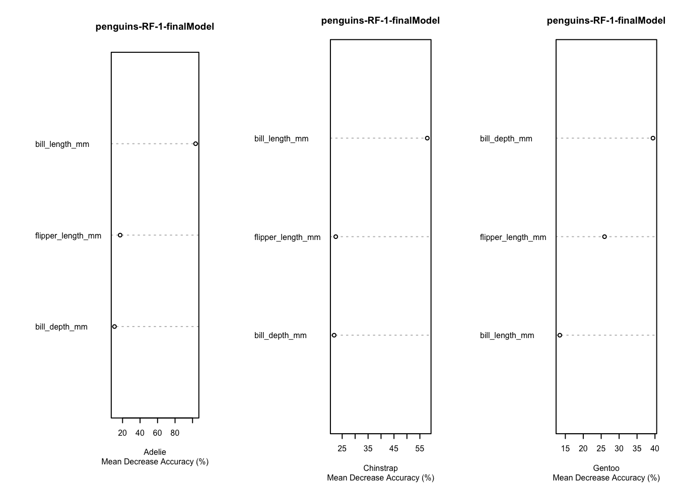
The best mtry parameter is 2. The (within-training) accuracy on the CV sample is 96.6%. On the test sample, the accuracy is 98%.
7.3.5 Sensitivity and Specificity: the basics
There are a lot of details given regarding the sensitivity and specificity of the procedure. They are broken down by outcome class (species, for penguins data). \[ \mbox{Sensitivity}_k = Pr(\mbox{Predict}=k\vert \mbox{Class}=k) \] \[ \mbox{Specificity}_k = Pr(\mbox{Predict}\neq k\vert\mbox{Class}\neq k) \] where \(k\) ranges over the \(K\) different levels of the nominal outcome (e.g., 3 penguins species). For example, Sensitivity of Chinstrap is 95%; the worst of the three, while Specificity for it is 98.7%, which is quite good. Our model “knows” when the features are not of a Chinstrap; it just has a harder time knowing that it is one.
7.4 ROC and AuC
Given a predictive model for the classification of nominal types, the predictions are typically probabilities of class membership.
- The decision to classify something as one type over another is known as a hard classification, and it is on this that most assessments are based. Typically, the maximum probability determines the choice.
- An option is to lower the probability at which a hard classifications is made; e.g., choosing one species over any other, we could decide affirmatively, whenever the predicted probability is above 0.10, 0.20, …, 0.50, 0.60, etc.
- The Receiver Operating Characteristic (ROC) curve is the True Positive Rate (TPR) vs. the False Positive Rate (FPR), and the curve is constructed by taking a wide range of alternative thresholds and calculating those two values for each.
- When the threshold is high, very few observations are declared positive, so the FPR is low, but so is the TPR.
- When the threshold is low, most observations are declared positive, so the TPR is high, but so is the FPR.
- The Area under the (ROC) curve (AuC) is the integral of the ROC curve from 0 to 1.
- Crash course:
- There is a probabilistic interpretation of AUC:
- The probability that randomly chosen positive example will be ranked higher (in probability of selection) than a randomly chosen negative example.
7.4.1 Variable importance
Variable importance for the penguins Data, based on the final model fit under cross-validation is given in these plots.
Code
par(mfrow=c(1,3))
for (i in 1:3) {
  varImpPlot(rf.penguins.1$finalModel,type=1,class=penguins.classes[i],main="penguins-RF-1-finalModel",sub="Mean Decrease Accuracy (%)",cex=.5)
}
Code
par(mfrow=c(1,1))7.4.2 Exercise 2
We now repeat the process, using the augmented feature set. We also make a much broader search through tuning parameters (for random forests, this is the number of predictors to try at each split). We allow for up to 9 predictors at each split. Best practice is to restrict the search to \(\sqrt{p}\) parameters at each stage, where \(p\) is the number of features. However, with only 9 features in the augmented space, we decided to see whether optimal tuning leads to more features than usual.
Code
set.seed(2011)
tuneGrid <- expand.grid(.mtry = c(1:9))  #as many as 18 variables in the data
rf.penguins.2 <- caret::train(species ~ bill_length_mm+bill_depth_mm+flipper_length_mm+BL.BD+FL.BD+BL.FL+BL.5+BD.5+FL.5, data=training, method = "rf", metric = "Accuracy", trControl = trControl, tuneGrid = tuneGrid, importance = TRUE, ntree = 300)
pred.rf.penguins.2 <-predict(rf.penguins.2, testing)
print(rf.penguins.2)
## Random Forest
##
## 235 samples
## 9 predictor
## 3 classes: 'Adelie', 'Chinstrap', 'Gentoo'
##
## No pre-processing
## Resampling: Cross-Validated (10 fold)
## Summary of sample sizes: 210, 212, 212, 212, 212, 213, ...
## Resampling results across tuning parameters:
##
## mtry Accuracy Kappa
## 1 0.9831377 0.9738309
## 2 0.9831377 0.9737690
## 3 0.9833188 0.9742146
## 4 0.9746232 0.9606852
## 5 0.9789710 0.9676098
## 6 0.9789710 0.9674137
## 7 0.9831377 0.9738687
## 8 0.9787899 0.9672020
## 9 0.9746232 0.9606267
##
## Accuracy was used to select the optimal model using the largest value.
## The final value used for the model was mtry = 3.Code
print(cm.penguins.2 <- confusionMatrix(pred.rf.penguins.2, testing$species))## Confusion Matrix and Statistics
##
## Reference
## Prediction Adelie Chinstrap Gentoo
## Adelie 42 2 0
## Chinstrap 1 18 0
## Gentoo 0 0 35
##
## Overall Statistics
##
## Accuracy : 0.9694
## 95% CI : (0.9131, 0.9936)
## No Information Rate : 0.4388
## P-Value [Acc > NIR] : < 2.2e-16
##
## Kappa : 0.9519
##
## Mcnemar's Test P-Value : NA
##
## Statistics by Class:
##
## Class: Adelie Class: Chinstrap Class: Gentoo
## Sensitivity 0.9767 0.9000 1.0000
## Specificity 0.9636 0.9872 1.0000
## Pos Pred Value 0.9545 0.9474 1.0000
## Neg Pred Value 0.9815 0.9747 1.0000
## Prevalence 0.4388 0.2041 0.3571
## Detection Rate 0.4286 0.1837 0.3571
## Detection Prevalence 0.4490 0.1939 0.3571
## Balanced Accuracy 0.9702 0.9436 1.0000Code
acc <- rf.penguins.2$results$Accuracy[best.ch <- which(as.numeric(rf.penguins.2$results$mtry)==as.numeric(rf.penguins.2$bestTune))]7.4.3 Discussion
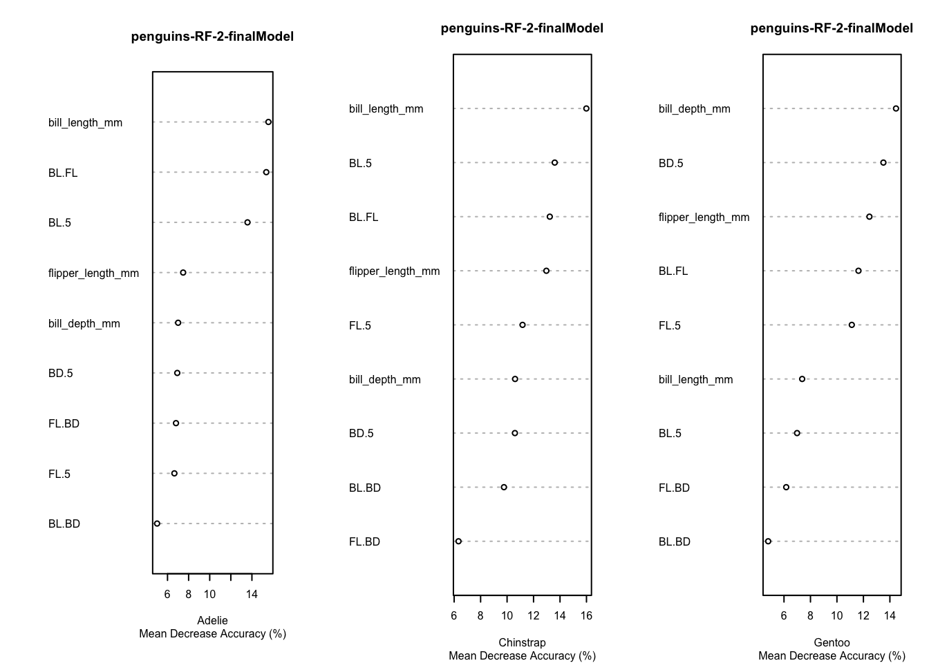
The best mtry parameter is 3. This is a little surprising, but we also had very good accuracy almost no matter what the mtry parameter. The (within-training) accuracy on the CV sample is 98.3%. On the test sample, the accuracy is 96.9%. This is a small test set, but it is interesting that no improvement occurred. Again, there are a lot of details given in the output regarding the sensitivity and specificity of the procedure.
7.5 Variable importance
Variable importance for the penguins Data, based on the final model fit under cross-validation is given in these plots.
Code
par(mfrow=c(1,3))
for (i in 1:3) {
  varImpPlot(rf.penguins.2$finalModel,type=1,class=penguins.classes[i],main="penguins-RF-2-finalModel",sub="Mean Decrease Accuracy (%)",cex=.5)
}
Code
par(mfrow=c(1,1))7.5.1 Random Forests with crabs data
We repeat the above procedure. First we run with the defaults, and the original 5 features.
Code
set.seed(2011)
inTrain <- createDataPartition(y=crabs$group, p=0.7, list=FALSE)
training <- crabs[inTrain,]
testing <- crabs[-inTrain,]
trControl <- trainControl(method = "cv", number = 10, search = "grid")
rf.crabs.1 <- caret::train(group ~ FL+RW+CL+CW+BD, data=training, method = "rf", metric = "Accuracy", trControl = trControl,importance = TRUE, ntree=300)
pred.rf.crabs.1 <-predict(rf.crabs.1, testing)
print(rf.crabs.1)
## Random Forest
##
## 140 samples
## 5 predictor
## 4 classes: 'Blue:Male', 'Blue:Female', 'Orange:Male', 'Orange:Female'
##
## No pre-processing
## Resampling: Cross-Validated (10 fold)
## Summary of sample sizes: 126, 126, 125, 128, 126, 126, ...
## Resampling results across tuning parameters:
##
## mtry Accuracy Kappa
## 2 0.7677839 0.6901889
## 3 0.7182601 0.6232247
## 5 0.7111172 0.6136765
##
## Accuracy was used to select the optimal model using the largest value.
## The final value used for the model was mtry = 2.Code
print(cm.crabs.1 <- confusionMatrix(pred.rf.crabs.1, testing$group))## Confusion Matrix and Statistics
##
## Reference
## Prediction Blue:Male Blue:Female Orange:Male Orange:Female
## Blue:Male 8 0 0 0
## Blue:Female 5 11 0 4
## Orange:Male 2 0 13 1
## Orange:Female 0 4 2 10
##
## Overall Statistics
##
## Accuracy : 0.7
## 95% CI : (0.5679, 0.8115)
## No Information Rate : 0.25
## P-Value [Acc > NIR] : 3.127e-13
##
## Kappa : 0.6
##
## Mcnemar's Test P-Value : NA
##
## Statistics by Class:
##
## Class: Blue:Male Class: Blue:Female Class: Orange:Male
## Sensitivity 0.5333 0.7333 0.8667
## Specificity 1.0000 0.8000 0.9333
## Pos Pred Value 1.0000 0.5500 0.8125
## Neg Pred Value 0.8654 0.9000 0.9545
## Prevalence 0.2500 0.2500 0.2500
## Detection Rate 0.1333 0.1833 0.2167
## Detection Prevalence 0.1333 0.3333 0.2667
## Balanced Accuracy 0.7667 0.7667 0.9000
## Class: Orange:Female
## Sensitivity 0.6667
## Specificity 0.8667
## Pos Pred Value 0.6250
## Neg Pred Value 0.8864
## Prevalence 0.2500
## Detection Rate 0.1667
## Detection Prevalence 0.2667
## Balanced Accuracy 0.7667Code
acc <- rf.crabs.1$results$Accuracy[best.ch <- which(as.numeric(rf.crabs.1$results$mtry)==as.numeric(rf.crabs.1$bestTune))]7.5.2 Discussion
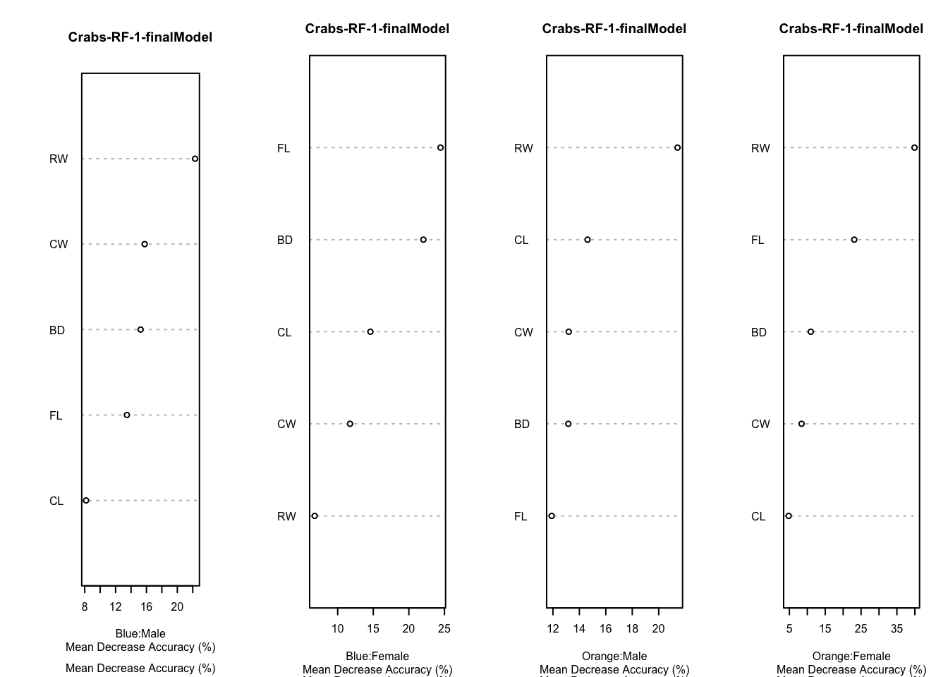
The best mtry parameter is 2. The (within-training) accuracy on the CV sample is 76.8%. On the test sample, the accuracy is 70%. There are a lot of details regarding the sensitivity and specificity of the procedure.
7.5.3 Variable importance
Variable importance for the Crabs Data, based on the final model fit under cross-validation is given in these plots.
Code
par(mfrow=c(1,4))
for (i in 1:4) {
  varImpPlot(rf.crabs.1$finalModel,type=1,class=crabs.classes[i],main="Crabs-RF-1-finalModel",sub="Mean Decrease Accuracy (%)",cex=.5)
}
Code
par(mfrow=c(1,1))We now repeat the process, using the augmented feature set. We also make a slightly broader search through tuning parameters. We allow for up to 7 predictors at each split. With only 7 features in the augmented space, we decided to see whether optimal tuning leads to more features than usual.
Code
set.seed(2011)
tuneGrid <- expand.grid(.mtry = c(1:7))  #as many as 7 variables in the data
rf.crabs.2 <- caret::train(group ~ FL+RW+CL+CW+BD+I(FL*RW)+I(CL*CW), data=training, method = "rf", metric = "Accuracy", trControl = trControl, tuneGrid = tuneGrid, importance = TRUE, ntree = 300)
pred.rf.crabs.2 <-predict(rf.crabs.2, testing)
print(rf.crabs.2)
## Random Forest
##
## 140 samples
## 5 predictor
## 4 classes: 'Blue:Male', 'Blue:Female', 'Orange:Male', 'Orange:Female'
##
## No pre-processing
## Resampling: Cross-Validated (10 fold)
## Summary of sample sizes: 125, 126, 128, 127, 125, 125, ...
## Resampling results across tuning parameters:
##
## mtry Accuracy Kappa
## 1 0.7273489 0.6330068
## 2 0.7185394 0.6220490
## 3 0.7200412 0.6243186
## 4 0.7190156 0.6224832
## 5 0.7052060 0.6046145
## 6 0.7344002 0.6436530
## 7 0.7278984 0.6354181
##
## Accuracy was used to select the optimal model using the largest value.
## The final value used for the model was mtry = 6.Code
print(cm.crabs.2 <- confusionMatrix(pred.rf.crabs.2, testing$group))## Confusion Matrix and Statistics
##
## Reference
## Prediction Blue:Male Blue:Female Orange:Male Orange:Female
## Blue:Male 8 0 1 0
## Blue:Female 5 11 0 4
## Orange:Male 2 0 13 0
## Orange:Female 0 4 1 11
##
## Overall Statistics
##
## Accuracy : 0.7167
## 95% CI : (0.5856, 0.8255)
## No Information Rate : 0.25
## P-Value [Acc > NIR] : 4.311e-14
##
## Kappa : 0.6222
##
## Mcnemar's Test P-Value : NA
##
## Statistics by Class:
##
## Class: Blue:Male Class: Blue:Female Class: Orange:Male
## Sensitivity 0.5333 0.7333 0.8667
## Specificity 0.9778 0.8000 0.9556
## Pos Pred Value 0.8889 0.5500 0.8667
## Neg Pred Value 0.8627 0.9000 0.9556
## Prevalence 0.2500 0.2500 0.2500
## Detection Rate 0.1333 0.1833 0.2167
## Detection Prevalence 0.1500 0.3333 0.2500
## Balanced Accuracy 0.7556 0.7667 0.9111
## Class: Orange:Female
## Sensitivity 0.7333
## Specificity 0.8889
## Pos Pred Value 0.6875
## Neg Pred Value 0.9091
## Prevalence 0.2500
## Detection Rate 0.1833
## Detection Prevalence 0.2667
## Balanced Accuracy 0.8111Code
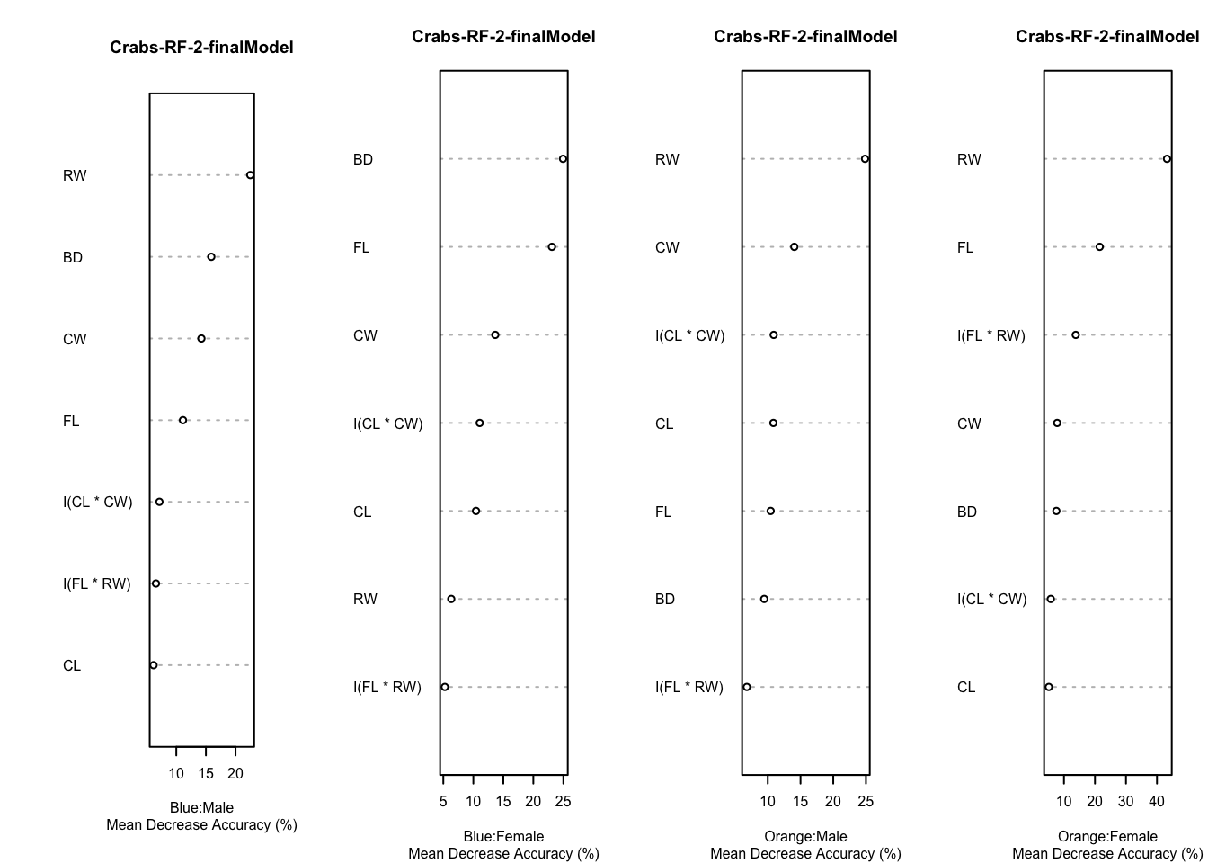
acc <- rf.crabs.2$results$Accuracy[best.ch <- which(as.numeric(rf.crabs.2$results$mtry)==as.numeric(rf.crabs.2$bestTune))]7.5.4 Discussion
The best mtry parameter is 6. This is equal to the choice when the feature set is smaller. Accuracy was better in sample, but slightly worse out of sample. The (within-training) accuracy on the CV sample is 73.4%. On the test sample, the accuracy is 71.7%. This isn’t very good, but this is the crabs data!
Code
par(mfrow=c(1,4))
for (i in 1:4) {
  varImpPlot(rf.crabs.2$finalModel,type=1,class=crabs.classes[i],main="Crabs-RF-2-finalModel",sub="Mean Decrease Accuracy (%)",cex=.5)
}
Code
par(mfrow=c(1,1))7.6 Neural Network (classification)
7.6.1 Some theory
Neural networks are a mathematical model for taking features, \(X=X_1,\ldots,X_P\) and transforming them (somehow) into outputs \(Y=Y_1,\ldots,Y_K\). Thus, we have \(P\) features and \(K\) outcomes. We will assume that the vector \(Y\) is the binary encoding of a categorical variable, such as penguins species (e.g., the first species is coded (1,0,0)). The classification problem translates to assigning probabilities to each level of this categorical variable. The simplest neural networks are multinomial logit models. These operate somewhat “simply”, as follows: \[T_k = \beta_{0k} + X\beta_k, \ \mbox{for}\ k=1,\ldots,K\] and \(\beta_k\) is a \(p\)-dimensional vector of coefficients. \(\beta_{0k}\) is a constant, often called the bias in neural networks. We define the vector \(T=T_1,\ldots,T_K\). Now the multinomial response (a binary vector \(Y\)) is modelled: \[P(Y_k) = g_k(T) = \frac{e^{T_k}}{\sum_{l=1}^K e^{T_l}}\] This is a variant of the multinomial logit formula, and \(\beta_k\) are multinomial regression coefficients.
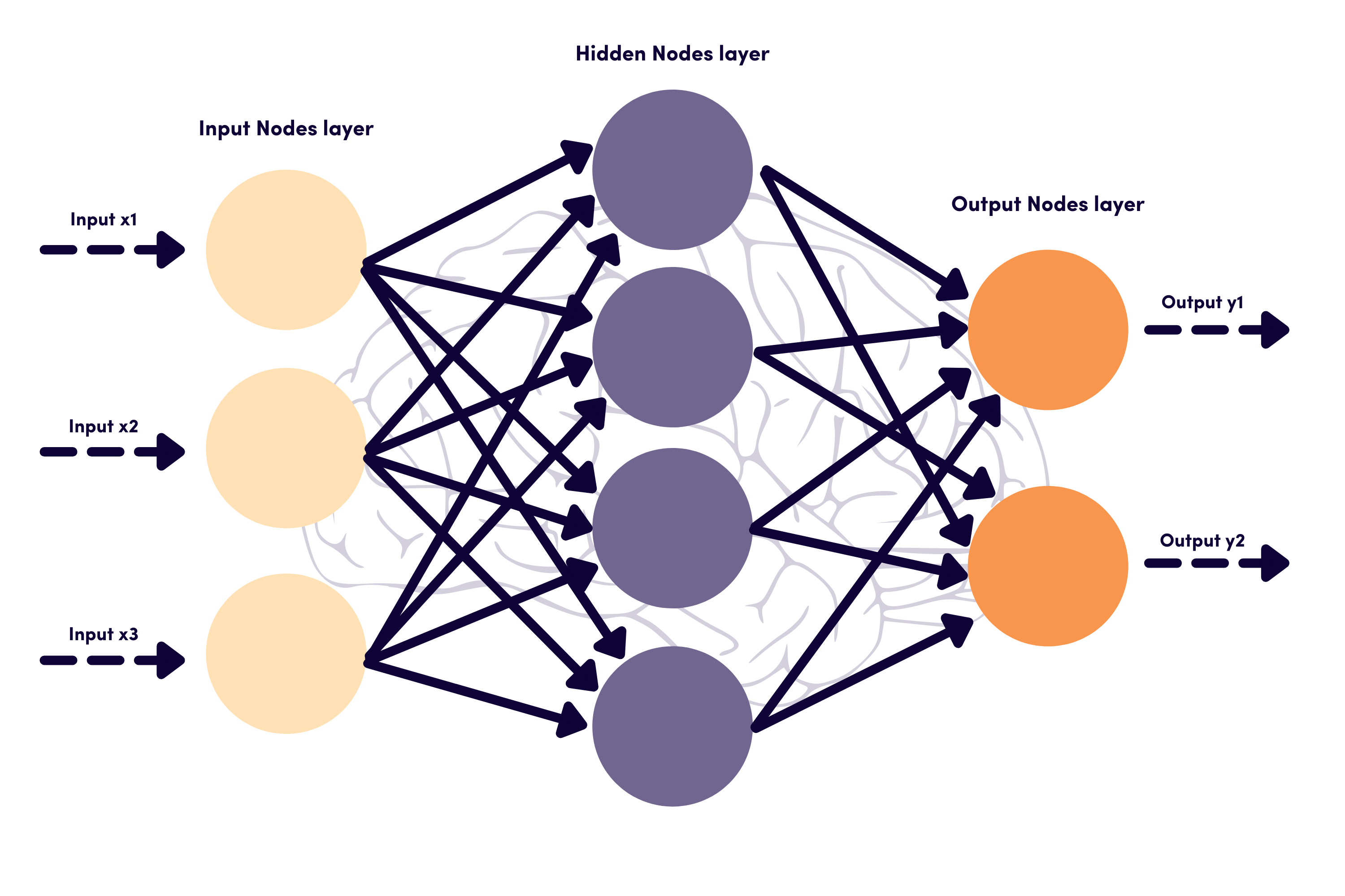
What makes a neural network able to “do more,” capturing nonlinear relationships between input \(X\) and output \(Y\) layers is the addition of one or more “hidden” layers that essentially recombine the original feature space into a new one, in a manner that is “learned” from the data.
A simple way to add one hidden layer, which is all that we will do here, is to rewrite the regression equation in terms of a set of hidden layer variables denotes \(Z\) as follows:
\[T_k = \beta_{0k} + Z\beta_k, \ \mbox{for}\ k=1,\ldots,K\] where \(Z=Z_1,\ldots,Z_M\), and \(M\) is the size of the hidden layer, and now \(\beta_k\) is an \(M\)-dimensional vector of regression coefficients on the hidden layer variables.
If the discussion so far bothers you, as \(Z\) is not observed directly, it both should and shouldn’t (bother you). It should bother you that we are regressing on unobserved variables. It shouldn’t bother you (too much), because we have built models using latent classes before (it’s the underlying construct of model-based clustering), and these weren’t observed either.
Code
xx <- neuraldat[, c("X1", "X2", "X3")]
yy <- neuraldat[, c("Y1", "Y2")]
mod1 <- mlp(xx,yy,size=4)
plotnet(mod1,cex=.55,rel_rsc=1.5)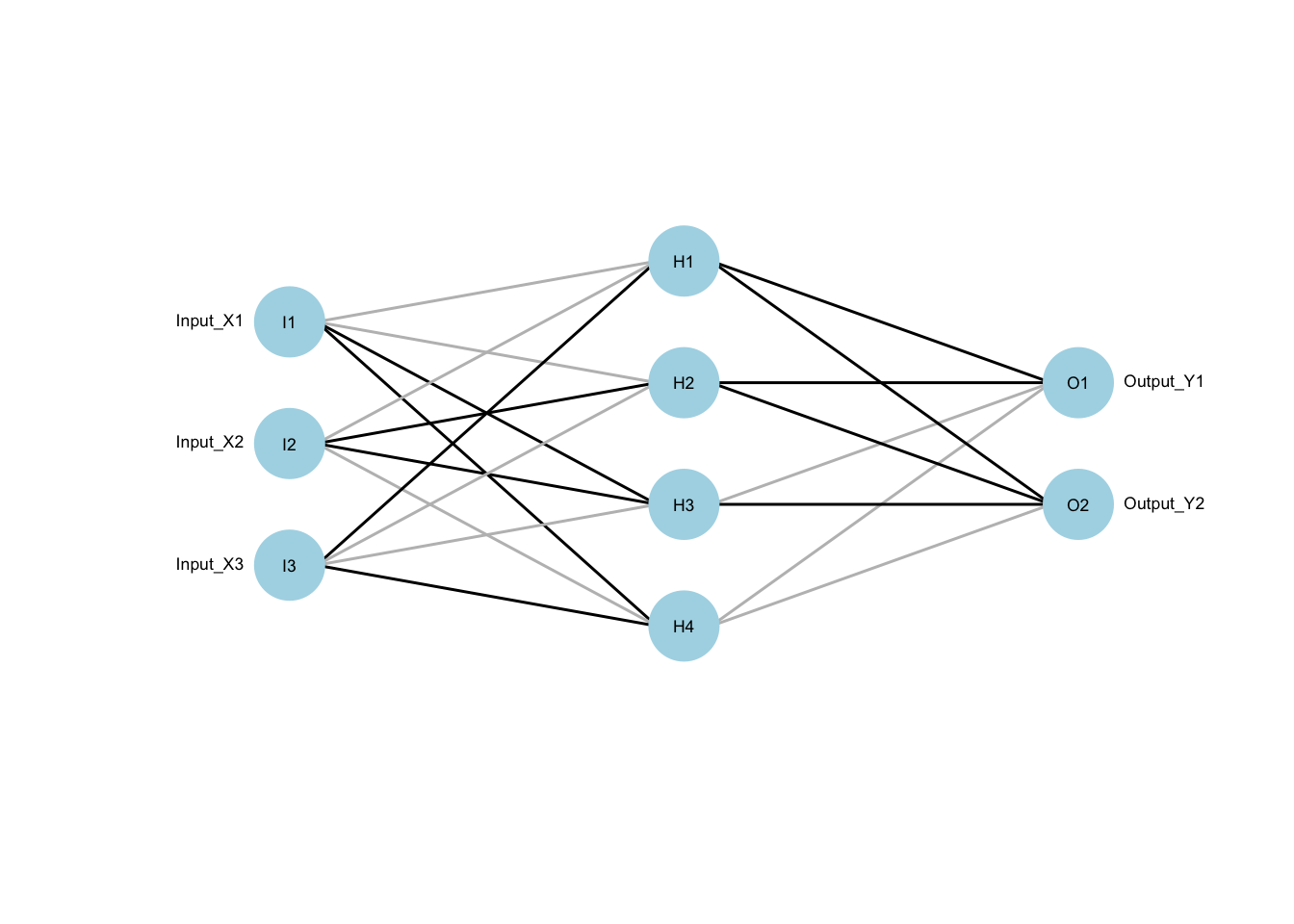
The diagram above should solidify the concepts. Nodes labelled I are input nodes (e.g., \(X_1,X_2,X_3\)), while the middle four nodes begin H as they are hidden, and to the right are output O nodes (e.g., \(Y_1,Y_2\)). That inner layer of hidden nodes allows for more complex relationships to be “learned.” We are calling these the Zs of our formal model.
We haven’t completed the mathematical model, though, as we need a way to transform \(X\) into \(Z\). This is where the lines between the nodes are used. Each is a weight coming from a coefficient vector. This equation completes the picture: \[Z_m = \sigma(\alpha_{0m}+X\alpha_m) \ \mbox{for}\ m=1,\ldots,M\] and \(\sigma\) is the “sigmoid” function we’ve been calling the inverse logit: \(\sigma(\nu)=\frac{e^\nu}{1+e^\nu}\). Other choices are possible, but this is a good place to start.
In terms of the figure, the lines between \(X\) and \(Z\) are weights given by many \(\alpha\) vectors. The sigmoid function transforms the weighted sum and stores the result in \(Z\). The lines between \(Z\) and \(Y\) are \(\beta\) vectors that generate \(T\) (a vector), which is transformed with the \(g(\cdot)\) function to a set of probabilities for categories in \(Y\). The bias terms \(\beta_{0k}\) are not included in this diagram.
7.6.2 Fitting a Neural Network (regularization)
The outcomes are multinomial draws, so we could write down a likelihood and maximize it. This would overtrain the model for the training data. Unfortunately, there is no simple equivalent to cross validation for the large parameter set. Instead, we use the notion of regularization, or penalized regression to avoid overfitting. We still use CV for choosing tuning parameters, but there are only a few of these. Maximizing the likelihood can be rewritten as a problem requiring minimization of deviance (think: sum of squares). Let’s call that deviance \(R(\theta)\), where \(\theta\) contains all of the parameters. Let \[J(\theta)=\sum_{km}\beta^2_{km} + \sum_{ml}\alpha^2_{ml}\] Then we seek to minimize \(R(\theta)+\lambda J(\theta)\), where \(\lambda\) is a tuning parameter. The larger \(\lambda\) is, the more parameters will be shrunk towards zero (rendering the path in the network to be nearly absent). The two tuning parameters in the implementation in the caret package are \(M\) and \(\lambda\), called size and decay in that software (note: decay may not be precisely \(\lambda\) as we have defined it here, but it has the same effect).
7.6.3 Application of neural networks to penguins data
We run two sets of neural networks, each with a single hidden layer. In the first, we use the three main penguins features and the default settings for the cross validation step. The defaults examine a hidden layers of sizes 1, 3 and 5, as well as decays of 0, 0.1 and 0.0001.
Code
set.seed(2011)
inTrain <- createDataPartition(y=penguins$species, p=0.7, list=FALSE)
training <- penguins[inTrain,]
testing <- penguins[-inTrain,]
trControl <- trainControl(method = "cv", number = 10, search = "grid")
text.nn.penguins.1 <- capture.output(nn.penguins.1 <- caret::train(species ~ bill_length_mm+bill_depth_mm+flipper_length_mm, data=training, method = "nnet", metric = "Accuracy", trControl = trControl,importance = TRUE))
pred.nn.penguins.1 <-predict(nn.penguins.1, testing)
print(nn.penguins.1)
## Neural Network
##
## 235 samples
## 3 predictor
## 3 classes: 'Adelie', 'Chinstrap', 'Gentoo'
##
## No pre-processing
## Resampling: Cross-Validated (10 fold)
## Summary of sample sizes: 211, 210, 213, 211, 212, 212, ...
## Resampling results across tuning parameters:
##
## size decay Accuracy Kappa
## 1 0e+00 0.4385323 0.0000000
## 1 1e-04 0.4385323 0.0000000
## 1 1e-01 0.7721621 0.6072475
## 3 0e+00 0.5668149 0.2296137
## 3 1e-04 0.6624671 0.4104960
## 3 1e-01 0.9829401 0.9730066
## 5 0e+00 0.4385323 0.0000000
## 5 1e-04 0.5343656 0.1671233
## 5 1e-01 0.9829401 0.9731329
##
## Accuracy was used to select the optimal model using the largest value.
## The final values used for the model were size = 3 and decay = 0.1.Code
print(cm.penguins.1 <- confusionMatrix(pred.nn.penguins.1, testing$species))## Confusion Matrix and Statistics
##
## Reference
## Prediction Adelie Chinstrap Gentoo
## Adelie 43 1 0
## Chinstrap 0 19 0
## Gentoo 0 0 35
##
## Overall Statistics
##
## Accuracy : 0.9898
## 95% CI : (0.9445, 0.9997)
## No Information Rate : 0.4388
## P-Value [Acc > NIR] : < 2.2e-16
##
## Kappa : 0.984
##
## Mcnemar's Test P-Value : NA
##
## Statistics by Class:
##
## Class: Adelie Class: Chinstrap Class: Gentoo
## Sensitivity 1.0000 0.9500 1.0000
## Specificity 0.9818 1.0000 1.0000
## Pos Pred Value 0.9773 1.0000 1.0000
## Neg Pred Value 1.0000 0.9873 1.0000
## Prevalence 0.4388 0.2041 0.3571
## Detection Rate 0.4388 0.1939 0.3571
## Detection Prevalence 0.4490 0.1939 0.3571
## Balanced Accuracy 0.9909 0.9750 1.0000Code
acc <- nn.penguins.1$results$Accuracy[best.ch <- as.numeric(dimnames(nn.penguins.1$bestTune)[[1]])]7.6.5 Discussion
The best (size,decay) parameters are (3,0.1). A decay of zero should mean no penalty, which potentially translates to overfitting. The (within-training) accuracy on the CV sample is 98.3%. On the test sample, the accuracy is 99%.
7.6.6 Visualization
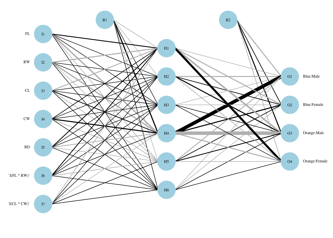
We are able to visualize this network, with the thickness of lines indicating their magnitude and the color indicating the sign (black=positive; grey=negative).
Code
par(mar=numeric(4),family='serif')
plotnet(nn.penguins.1$finalModel, cex_val=.5,neg_col="red",pos_col="green")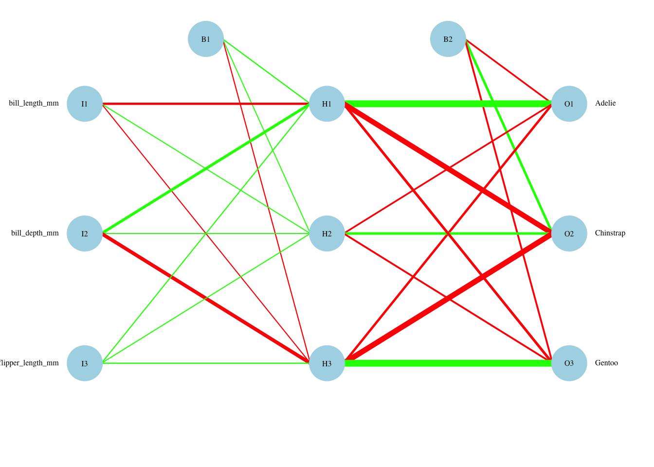
Following the paths, it is clear that bill depth represents most of the information in hidden nodes H1 and H3. Bill length feeds strongly into hidden node H2. Using the coloring, H1 influences the choice favoring Adelie positively, while H2 does so negatively. H3 influences the choice favoring Chinstrap positively, while H1 does so negatively, and finally, H2 influences the choice favoring Gentoo positively, while H3 does so negatively. These are more complex influences than a standard linear model due to the sigmoid function non-linear transformation and the potential interaction effects captured in the hidden layer.
We now repeat the fitting process using the (much) larger feature set and search through tuning parameters on a grid with sizes 1-9 and weight decay between 0 and 0.1 by 0.025, as well as testing 0.01 (a total of 6 values for decay).
Code
set.seed(2011)
tuneGrid <- expand.grid(.size = c(1:9), .decay=c(0,2.5e-2,5e-2,7.5e-2,1e-1,1e-2) )
text.nn.penguins.2 <- capture.output(nn.penguins.2 <- caret::train(species ~ bill_length_mm+bill_depth_mm+flipper_length_mm+BL.BD+FL.BD+BL.FL+BL.5+BD.5+FL.5, data=training, method = "nnet", metric = "Accuracy", trControl = trControl, tuneGrid = tuneGrid, importance = TRUE))
pred.nn.penguins.2 <-predict(nn.penguins.2, testing)
print(nn.penguins.2)
## Neural Network
##
## 235 samples
## 9 predictor
## 3 classes: 'Adelie', 'Chinstrap', 'Gentoo'
##
## No pre-processing
## Resampling: Cross-Validated (10 fold)
## Summary of sample sizes: 210, 212, 212, 212, 212, 213, ...
## Resampling results across tuning parameters:
##
## size decay Accuracy Kappa
## 1 0.000 0.4383458 0.00000000
## 1 0.010 0.5253024 0.15662639
## 1 0.025 0.5771285 0.25060547
## 1 0.050 0.5723458 0.24666207
## 1 0.075 0.7272372 0.52870641
## 1 0.100 0.5426937 0.19154335
## 2 0.000 0.4383458 0.00000000
## 2 0.010 0.7760507 0.60989590
## 2 0.025 0.7285125 0.51714050
## 2 0.050 0.5735125 0.24458021
## 2 0.075 0.7173386 0.50276556
## 2 0.100 0.8221014 0.68691622
## 3 0.000 0.4731285 0.06439628
## 3 0.010 0.8338096 0.71109359
## 3 0.025 0.8202681 0.68583123
## 3 0.050 0.8425507 0.73028123
## 3 0.075 0.8492009 0.73989377
## 3 0.100 0.8993966 0.83264902
## 4 0.000 0.4383458 0.00000000
## 4 0.010 0.9447319 0.90863532
## 4 0.025 0.8642589 0.76625887
## 4 0.050 0.9157299 0.85405583
## 4 0.075 0.7982826 0.64686307
## 4 0.100 0.9608531 0.93568557
## 5 0.000 0.4383458 0.00000000
## 5 0.010 0.7571430 0.57728947
## 5 0.025 0.9233116 0.86917874
## 5 0.050 0.9161087 0.85989477
## 5 0.075 0.9570507 0.93180484
## 5 0.100 0.9355072 0.89516427
## 6 0.000 0.4503458 0.02948718
## 6 0.010 0.7863986 0.63184823
## 6 0.025 0.9528841 0.92460074
## 6 0.050 0.9282444 0.87297900
## 6 0.075 0.9499710 0.91927136
## 6 0.100 0.8918333 0.81706911
## 7 0.000 0.5091285 0.13132750
## 7 0.010 0.8746232 0.78928672
## 7 0.025 0.9784420 0.96627346
## 7 0.050 0.9664420 0.94675482
## 7 0.075 0.9661087 0.94681256
## 7 0.100 0.9570652 0.93287652
## 8 0.000 0.4731285 0.06461538
## 8 0.010 0.8981080 0.82918268
## 8 0.025 0.9309638 0.88028950
## 8 0.050 0.9701087 0.95335130
## 8 0.075 0.9287734 0.87319576
## 8 0.100 0.9660942 0.94742873
## 9 0.000 0.4964486 0.11385532
## 9 0.010 0.9704565 0.95327240
## 9 0.025 0.9659275 0.94407133
## 9 0.050 0.9454420 0.91188619
## 9 0.075 0.9671377 0.94583653
## 9 0.100 0.9873188 0.97957501
##
## Accuracy was used to select the optimal model using the largest value.
## The final values used for the model were size = 9 and decay = 0.1.Code
print(cm.penguins.2 <- confusionMatrix(pred.nn.penguins.2, testing$species))## Confusion Matrix and Statistics
##
## Reference
## Prediction Adelie Chinstrap Gentoo
## Adelie 43 1 1
## Chinstrap 0 16 0
## Gentoo 0 3 34
##
## Overall Statistics
##
## Accuracy : 0.949
## 95% CI : (0.8849, 0.9832)
## No Information Rate : 0.4388
## P-Value [Acc > NIR] : <2e-16
##
## Kappa : 0.9191
##
## Mcnemar's Test P-Value : 0.1718
##
## Statistics by Class:
##
## Class: Adelie Class: Chinstrap Class: Gentoo
## Sensitivity 1.0000 0.8000 0.9714
## Specificity 0.9636 1.0000 0.9524
## Pos Pred Value 0.9556 1.0000 0.9189
## Neg Pred Value 1.0000 0.9512 0.9836
## Prevalence 0.4388 0.2041 0.3571
## Detection Rate 0.4388 0.1633 0.3469
## Detection Prevalence 0.4592 0.1633 0.3776
## Balanced Accuracy 0.9818 0.9000 0.9619Code
acc <- nn.penguins.2$results$Accuracy[best.ch <- as.numeric(dimnames(nn.penguins.2$bestTune)[[1]])]7.6.7 Discussion
The best (size,decay) parameters are (9,0.1). The (within-training) accuracy on the CV sample is 98.7%. On the test sample, the accuracy is 94.9%. There was some improvement in withheld test sample accuracy with the additional feature set, but surprisingly the hidden layer shrunk to a single node. This suggests that the expanded feature set captures much of the non-linearity needed to accurately model penguins data.
7.7 Visualization
We are able to visualize this network as well.
Code
par(mar=numeric(4),family='serif')
plotnet(nn.penguins.2$finalModel, cex_val=.5,neg_col="red",pos_col="green")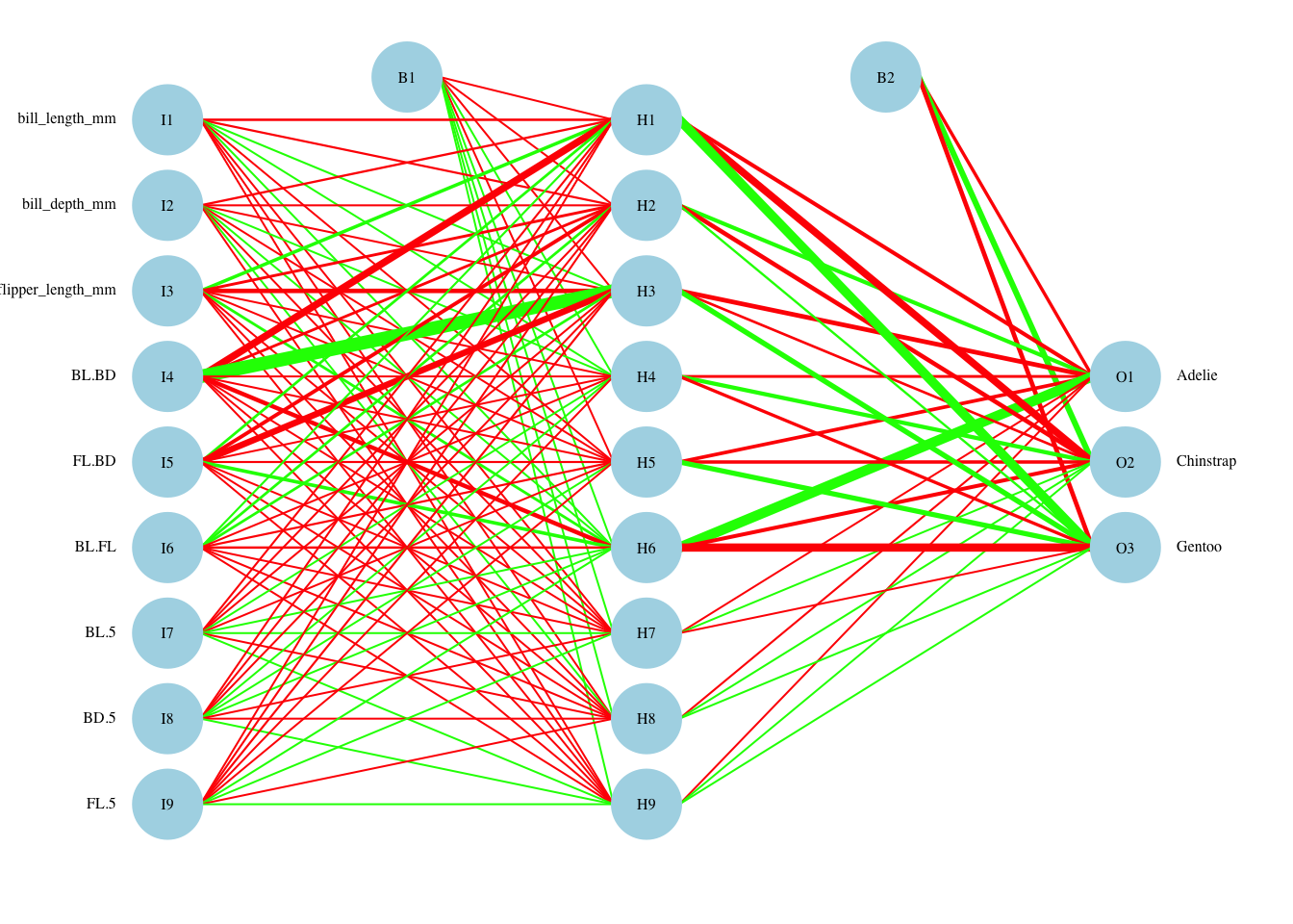 What happened here? We have introduced many non-linear (or at least complex) terms in the feature space, and many are used in prediction. There are some hidden layers that receive only positive inputs, and the opposite. A smaller number of hidden layers seem to have the largest impact on the outcome, so one would think that we could use a smaller hidden layer. In fact, 4 hidden nodes seems to perform about as well, but when we redo the grid search, differences that cannot be controlled by seed setting move away from the optimal setting for 4 nodes.
7.7.1 Neural Network with crabs data:
We repeat the above procedure. First we run with the defaults, and the original 5 features. Then we add two interaction terms.
Code
set.seed(2011)
inTrain <- createDataPartition(y=crabs$group, p=0.7, list=FALSE)
training <- crabs[inTrain,]
testing <- crabs[-inTrain,]
trControl <- trainControl(method = "cv", number = 10, search = "grid")
text.nn.crabs.1 <- capture.output(nn.crabs.1 <- caret::train(group~FL+RW+CL+CW+BD, data=training, method = "nnet", metric = "Accuracy", trControl = trControl,importance = TRUE))
pred.nn.crabs.1 <-predict(nn.crabs.1, testing)
print(nn.crabs.1)
## Neural Network
##
## 140 samples
## 5 predictor
## 4 classes: 'Blue:Male', 'Blue:Female', 'Orange:Male', 'Orange:Female'
##
## No pre-processing
## Resampling: Cross-Validated (10 fold)
## Summary of sample sizes: 126, 126, 125, 128, 126, 126, ...
## Resampling results across tuning parameters:
##
## size decay Accuracy Kappa
## 1 0e+00 0.1865568 -0.03656566
## 1 1e-04 0.4068864 0.24417790
## 1 1e-01 0.7807326 0.70908310
## 3 0e+00 0.3383150 0.15578514
## 3 1e-04 0.6076007 0.48868454
## 3 1e-01 0.9426374 0.92361650
## 5 0e+00 0.7680220 0.69852839
## 5 1e-04 0.8573077 0.81409002
## 5 1e-01 0.9651648 0.95353151
##
## Accuracy was used to select the optimal model using the largest value.
## The final values used for the model were size = 5 and decay = 0.1.Code
print(cm.crabs.1 <- confusionMatrix(pred.nn.crabs.1, testing$group))## Confusion Matrix and Statistics
##
## Reference
## Prediction Blue:Male Blue:Female Orange:Male Orange:Female
## Blue:Male 12 0 0 0
## Blue:Female 3 15 0 0
## Orange:Male 0 0 15 0
## Orange:Female 0 0 0 15
##
## Overall Statistics
##
## Accuracy : 0.95
## 95% CI : (0.8608, 0.9896)
## No Information Rate : 0.25
## P-Value [Acc > NIR] : < 2.2e-16
##
## Kappa : 0.9333
##
## Mcnemar's Test P-Value : NA
##
## Statistics by Class:
##
## Class: Blue:Male Class: Blue:Female Class: Orange:Male
## Sensitivity 0.8000 1.0000 1.00
## Specificity 1.0000 0.9333 1.00
## Pos Pred Value 1.0000 0.8333 1.00
## Neg Pred Value 0.9375 1.0000 1.00
## Prevalence 0.2500 0.2500 0.25
## Detection Rate 0.2000 0.2500 0.25
## Detection Prevalence 0.2000 0.3000 0.25
## Balanced Accuracy 0.9000 0.9667 1.00
## Class: Orange:Female
## Sensitivity 1.00
## Specificity 1.00
## Pos Pred Value 1.00
## Neg Pred Value 1.00
## Prevalence 0.25
## Detection Rate 0.25
## Detection Prevalence 0.25
## Balanced Accuracy 1.00Code
acc <- nn.crabs.1$results$Accuracy[best.ch <- as.numeric(dimnames(nn.crabs.1$bestTune)[[1]])]7.7.2 Discussion
The best (size,decay) parameters are (5,0.1). The (within-training) accuracy on the CV sample is 96.5%. On the test sample, the accuracy is 95%.
7.7.3 Visualization
Code
par(mar=numeric(4),family='serif')
plotnet(nn.crabs.1$finalModel, cex_val=.5)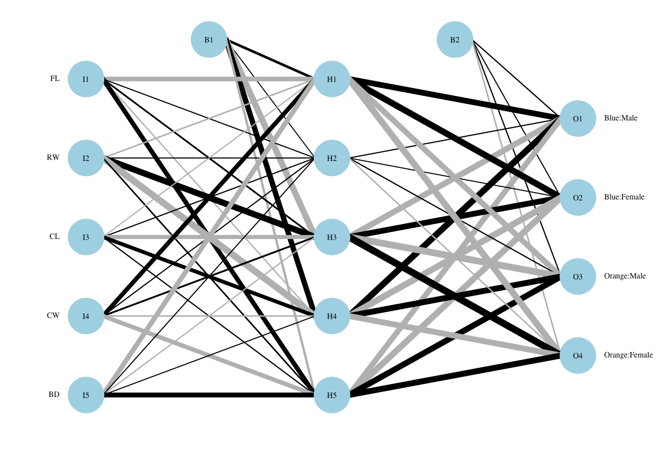
While it is difficult to interpret this network, we can see that all nodes in the hidden layer play some role both from the original feature set to the output layer.
We now repeat the fitting process using the (slightly) larger feature set and search through tuning parameters on a grid with sizes 1-7 and weight decay between 0 and 0.1 by 0.025, as well as testing 0.01 (a total of 6 values for decay).
Code
set.seed(2011)
tuneGrid <- expand.grid(.size = c(1:7), .decay=c(0,2.5e-2,5e-2,7.5e-2,1e-1,1e-2) )
text.nn.crabs.2 <- capture.output(nn.crabs.2 <- caret::train(group~FL+RW+CL+CW+BD+I(FL*RW)+I(CL*CW), data=training, method = "nnet", metric = "Accuracy", trControl = trControl, tuneGrid = tuneGrid, importance = TRUE))
pred.nn.crabs.2 <-predict(nn.crabs.2, testing)
print(nn.crabs.2)
## Neural Network
##
## 140 samples
## 5 predictor
## 4 classes: 'Blue:Male', 'Blue:Female', 'Orange:Male', 'Orange:Female'
##
## No pre-processing
## Resampling: Cross-Validated (10 fold)
## Summary of sample sizes: 125, 126, 128, 127, 125, 125, ...
## Resampling results across tuning parameters:
##
## size decay Accuracy Kappa
## 1 0.000 0.1759478 -0.061666667
## 1 0.010 0.6306364 0.519459410
## 1 0.025 0.6292399 0.520192347
## 1 0.050 0.8018223 0.734729637
## 1 0.075 0.7642353 0.684843183
## 1 0.100 0.5945238 0.465263459
## 2 0.000 0.2204991 -0.002777778
## 2 0.010 0.7564698 0.677936806
## 2 0.025 0.7747207 0.701632951
## 2 0.050 0.8513141 0.800532536
## 2 0.075 0.7721978 0.702913698
## 2 0.100 0.7436447 0.660108988
## 3 0.000 0.2928663 0.093535354
## 3 0.010 0.8233974 0.764876429
## 3 0.025 0.9057143 0.874819721
## 3 0.050 0.9108929 0.881589726
## 3 0.075 0.8581502 0.811451906
## 3 0.100 0.9133333 0.884599984
## 4 0.000 0.2375092 0.019292929
## 4 0.010 0.8666392 0.821780451
## 4 0.025 0.8550366 0.808423513
## 4 0.050 0.9154212 0.887655267
## 4 0.075 0.9653571 0.953822673
## 4 0.100 0.8751282 0.831933263
## 5 0.000 0.2517674 0.033060841
## 5 0.010 0.7880769 0.717342414
## 5 0.025 0.8933654 0.857749767
## 5 0.050 0.8970238 0.862764159
## 5 0.075 0.8784020 0.837271879
## 5 0.100 0.9360577 0.914184531
## 6 0.000 0.2670421 0.054752442
## 6 0.010 0.9229487 0.897187392
## 6 0.025 0.9711905 0.961389240
## 6 0.050 0.9279487 0.903624260
## 6 0.075 0.8918956 0.856821006
## 6 0.100 0.9558059 0.940813600
## 7 0.000 0.2530998 0.040353535
## 7 0.010 0.8459707 0.794174508
## 7 0.025 0.8937683 0.856404581
## 7 0.050 0.9159386 0.888142860
## 7 0.075 0.9022527 0.868785045
## 7 0.100 0.9211630 0.894823756
##
## Accuracy was used to select the optimal model using the largest value.
## The final values used for the model were size = 6 and decay = 0.025.Code
print(cm.crabs.2 <- confusionMatrix(pred.nn.crabs.2, testing$group))## Confusion Matrix and Statistics
##
## Reference
## Prediction Blue:Male Blue:Female Orange:Male Orange:Female
## Blue:Male 12 1 0 0
## Blue:Female 3 12 1 0
## Orange:Male 0 0 14 1
## Orange:Female 0 2 0 14
##
## Overall Statistics
##
## Accuracy : 0.8667
## 95% CI : (0.7541, 0.9406)
## No Information Rate : 0.25
## P-Value [Acc > NIR] : < 2.2e-16
##
## Kappa : 0.8222
##
## Mcnemar's Test P-Value : NA
##
## Statistics by Class:
##
## Class: Blue:Male Class: Blue:Female Class: Orange:Male
## Sensitivity 0.8000 0.8000 0.9333
## Specificity 0.9778 0.9111 0.9778
## Pos Pred Value 0.9231 0.7500 0.9333
## Neg Pred Value 0.9362 0.9318 0.9778
## Prevalence 0.2500 0.2500 0.2500
## Detection Rate 0.2000 0.2000 0.2333
## Detection Prevalence 0.2167 0.2667 0.2500
## Balanced Accuracy 0.8889 0.8556 0.9556
## Class: Orange:Female
## Sensitivity 0.9333
## Specificity 0.9556
## Pos Pred Value 0.8750
## Neg Pred Value 0.9773
## Prevalence 0.2500
## Detection Rate 0.2333
## Detection Prevalence 0.2667
## Balanced Accuracy 0.9444Code
acc <- nn.crabs.2$results$Accuracy[best.ch <- as.numeric(dimnames(nn.crabs.2$bestTune)[[1]])]7.7.4 Discussion
The best (size,decay) parameters are (6,0.025). The (within-training) accuracy on the CV sample is 97.1%. On the test sample, the accuracy is 86.7%. There was loss of accuracy in the withheld test sample accuracy with the additional feature set, and the hidden layer grew to 7 nodes.
Perhaps this underscores that:
- Neural nets do well with original feature space and do not “require” as much feature augmentation (this is theoretically handled by the hidden layers).
- The size of the hidden layer matters. Perhaps we overfit somewhat, through the hidden layer nodes.