5 Chapter 5: Support Vector Machines (SVMs)
5.1 Introduction
- SVMs are meant to be ‘trainable’ classifiers that operate on new (or withheld) data with the goal of optimal prediction (not description)
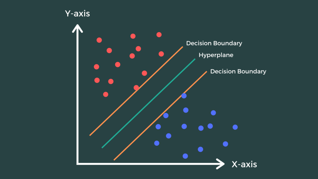
- When you have well-separated groups, a line (or plane in higher dimensions) will perfectly separate observations in one group from the others.
- There is no unique solution: more than one line will separate two groups.
- Imposing an additional constraint, that the line must maximize the gap or margin between the observations closest to it, makes it identifiable.
- This formulation leads to computational efficiencies, since the actual number of observations needed to determine the optimal line tends to be small
- Good for training, ‘storage’ and then later prediction
- These points are known as the support vectors.
- When the groups are not perfectly separated, the equations that govern the separating line can be easily modified to handle the case.
- Extensions of the approach have proven to be very effective
- Use of kernels; more than two groups.
5.1.1 Example: Penguins as a two group discrimination problem
- Merge Adelie and Chinstrap
- Restrict the analysis to 2-D
- Use Bill Depth and Flipper Width to discriminate.
- ‘helper’ function visible in Rmd only. It plots an approximate version of the margin.
Code
# sepLinePlot signature:  function(svm.fit,data,target=data$species,cols=c(2,3)) ...
penguins_12_3 <- penguins %>% mutate(species=dplyr::recode(species,`Adelie`="Adel/Chin",`Chinstrap`="Adel/Chin"))
5.2 SVM in the linear, separable case
Code
sv.fit.lin0 <- e1071::svm(species ~ bill_depth_mm+flipper_length_mm, data = penguins_12_3,kernel='linear')
sepLinePlot(sv.fit.lin0,penguins_12_3)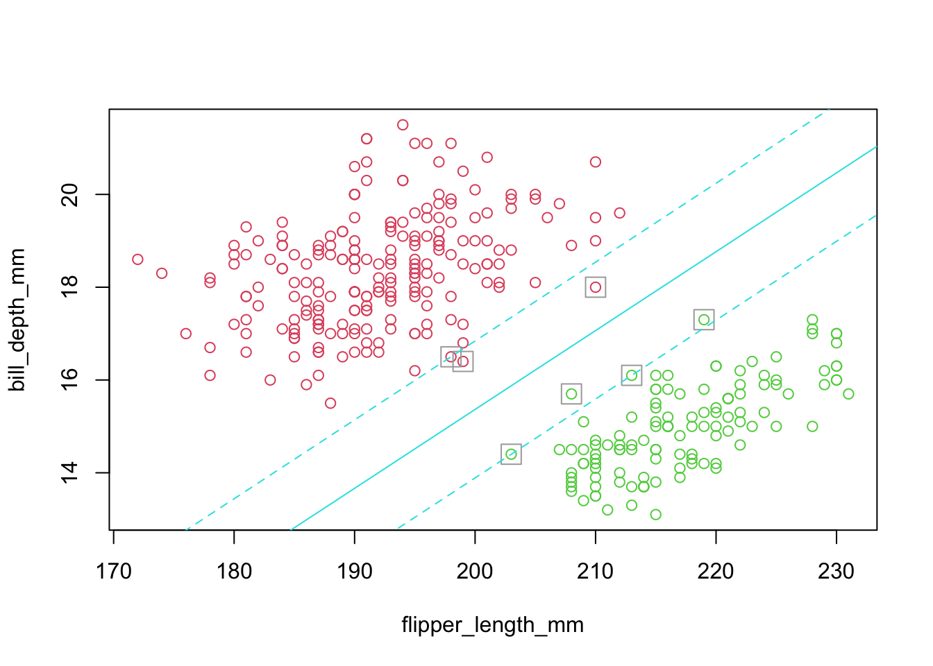
5.2.2 Notes
- Solid line is the separating (hyper)plane.
- Margins are dashed.
- The margin is constructed by widening the line until it just touches points (called support vectors) on either side.
- With edges parallel to the separating plane.
5.2.4 Example: penguins Ignoring Gentoo (non-separable case)
- Imperfectly separated groups
- Restrict the analysis to 2-D
- Use Bill Length and Depth to discriminate
- However, there is no ‘clean’ separating line.
- The algorithm handles for this case by incorporating ‘slack’ or some amount of crossover in the margin (details will follow).
Code
penguins_1_2 <- penguins %>% filter(species!="Gentoo")
sv.fit.lin <- svm(species ~ bill_length_mm+bill_depth_mm, data = penguins_1_2,kernel='linear')
sepLinePlot(sv.fit.lin,penguins_1_2)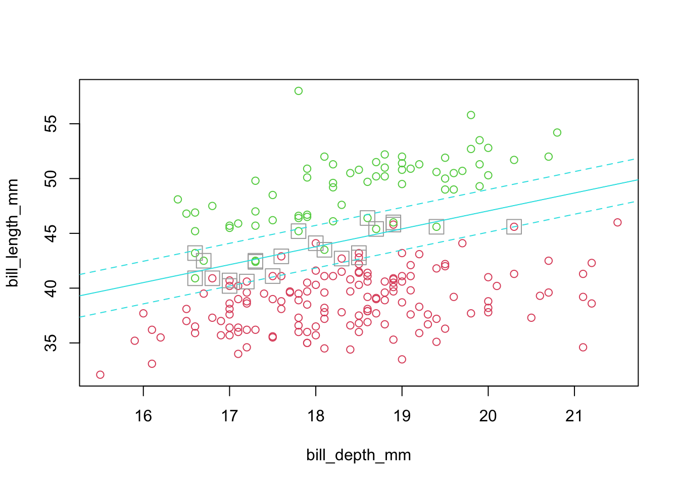
5.3 Derivation of the SVM approach to classification
- We are given a p-dimensional feature set \({{X}_{1i}},{{X}_{2i}},\ldots ,{{X}_{pi}}\) for observation \(i\), and two groups defined as the outcome \({{Y}_{i}}\in \{-1,+1\}\), where those values indicate the group label
- This convention simplifies some math later on
- A class of hyperplanes (think: lines in 2-D), is defined by \({{\beta }_{0}}+{{\beta }_{1}}{{X}_{1i}}+{{\beta }_{2}}{{X}_{2i}}+\ldots +{{\beta }_{p}}{{X}_{pi}}=0\)
- In 2-D, these can be rewritten in ‘y=mx+b’ form as \({{X}_{2}}=-\frac{\beta_0}{\beta_2}-\frac{{{\beta }_{1}}}{{{\beta }_{2}}}{{X}_{1}}\).
- Define \(F(\vec{X})={{\beta }_{0}}+{{\beta }_{1}}{{X}_{1}}+{{\beta }_{2}}{{X}_{2}}+\ldots +{{\beta }_{p}}{{X}_{p}}\)
- where \(\vec{X}=[{{X}_{1}},{{X}_{2}},\ldots ,{{X}_{p}}{]}'\) is a vector
- Think of each observation, which is a collection of features, as one such vector \({{\vec{X}}_{i}}\).
- Then \(F({{\vec{X}}_{i}})>0\) or \(F({{\vec{X}}_{i}})<0\) depending on which side of the hyperplane \({{\vec{X}}_{i}}\) lies.
- By proper assignment of \({{Y}_{i}}\in \{-1,+1\}\), the value of \({{Y}_{i}}\cdot F({{\vec{X}}_{i}})>0\) for all \(i\), if a separating hyperplane exists.
- When the groups are perfectly separable, then the goal is to maximize \(M\), the margin, over values of \(\vec{\beta }=[{{\beta }_{0}},{{\beta }_{1}},{{\beta }_{2}},\ldots ,{{\beta }_{p}}{]}'\), subject to constraints.
- The constraints are:
- \({{\left\| {\vec{\beta }} \right\|}^{2}}=\sum\limits_{i=1}^{p}{\beta_{i}^{2}}=1\) (for identifiability)
- \(\forall i\), \({{Y}_{i}}\cdot F({{\vec{X}}_{i}})={{Y}_{i}}\cdot ({{\beta }_{0}}+{{\beta }_{1}}{{X}_{1i}}+{{\beta }_{2}}{{X}_{2i}}+\ldots +{{\beta }_{p}}{{X}_{pi}})\ge M\).
This last line says that all points lie outside the margin (we will have to relax this for non-separable cases).
- This maximization problem is well understood and software exists to solve it efficiently.
- Note, however, that the implementation of svm in R uses a slightly different, but equivalent set of constraints.
- The constraints are:
5.3.1 Case: groups are non-separable
- We modify the maximization problem, adding many parameters and in particular a cost, \(C\), known as a regularization parameter.
- To get this problem formulation to conform more closely to the literature, we reframe it as this minimization problem:
- We want \(\underset{{{\beta }_{0}},\vec{\beta },\vec{\varepsilon },M}{\mathop{\min }}\,\frac{{\vec{\beta }}'\vec{\beta }}{M}+C\sum\limits_{i=1}^{N}{{{\varepsilon }_{i}}}\) Such that \({{\left\| {\vec{\beta }} \right\|}^{2}}= 1\), \({{\varepsilon }_{i}} \ge 0\), and \[\begin{eqnarray*} {{Y}_{i}}\cdot F({{\vec{X}}_{i}}) & = & {{Y}_{i}}\cdot ({{\beta }_{0}}+{{\beta }_{1}}{{X}_{1i}}+{{\beta }_{2}}{{X}_{2i}}+\ldots +{{\beta }_{p}}{{X}_{pi}})\ge M(1-{{\varepsilon }_{i}}) \end{eqnarray*}\] \(\forall i = 1,\ldots,N.\)
- To get this problem formulation to conform more closely to the literature, we reframe it as this minimization problem:
5.4 Slack
- Each element of the vector \(\vec{\varepsilon }=[{{\varepsilon }_{1}},\ldots ,{{\varepsilon }_{n}}{]}'\) is known as slack for that observation.
- They are essentially the distance of each point from the margin for that group.
- They are allowances for observations that are on the ‘wrong side’ of the separating plane and are similar to residuals in regression.
- They are essentially the distance of each point from the margin for that group.
- Slack \({{\varepsilon }_{i}}=0\) when point \(i\) is on the proper side of the margin.
- Slack \(0<{{\varepsilon }_{i}}\le 1\) when point \(i\) is on the proper side of the separating plane, but within the margin.
- They are classified correctly, but recall that with separable groups, no observation in within the margin.
- Slack \({{\varepsilon }_{i}}>1\) when point \(i\) is on the wrong side of the separating plane.
- The margin \(M\) and cost \(C\) work together to constrain the use of slack.
- In our formulation, decreasing the cost \(C\) provides more slack and more support vectors.
5.4.1 Example (cont.)
- We have tried to have the above formulation correspond to the implementation in R’s svm implementation in package e1071.
- We use cost \(C\) to change the separating plane and show its consequences.
- Here is the last svm classification based on the default cost \(C=1\) for the second example, with several misclassified observations:
Code
plot(sv.fit.lin,penguins_1_2,formula=bill_depth_mm ~ bill_length_mm)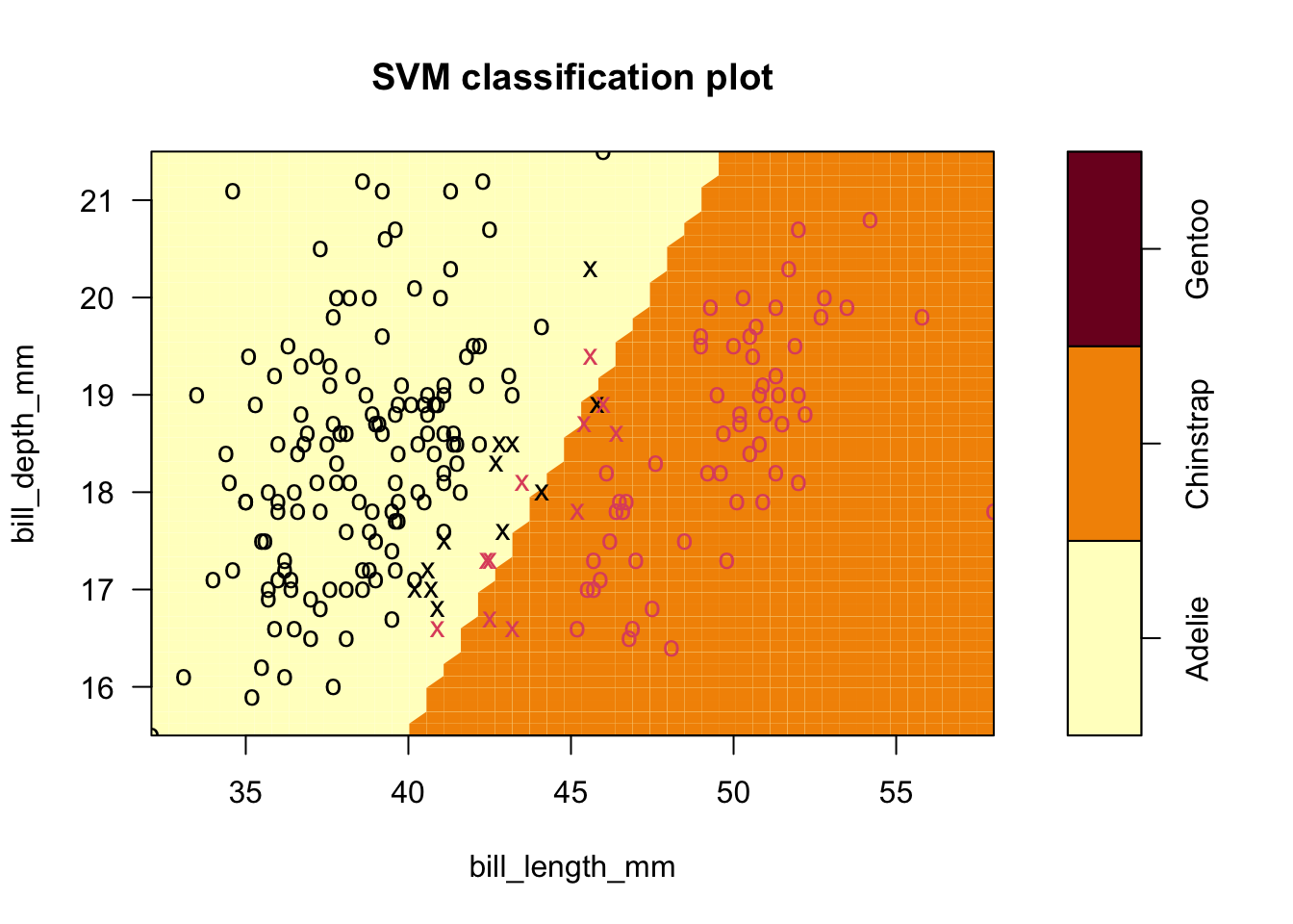
5.4.2 Notes
- In this plot, group membership is given by the symbol color so you can see seven misclassified observations.
- The symbol is ‘o’ when it is not a support vector (SV), and ‘x’ when it is.
- In this plot, you can see that there are a fairly large number of support vectors
- Contrast this to the seven SVs in the completely separable case.
- In this plot, you can see that there are a fairly large number of support vectors
- Now decrease \(C\) so that the margin \(M\) must shrink to accommodate the slack in the misclassified observations.
- This will increase the number of SVs used.
- The advantage to decreasing \(C\), and thus increasing the number of SVs, is that the separating plane is less susceptible to a few outlying observations.
- Results shown next for C=0.01
Code
sv.fit.lin.lowCost <- svm(species ~ bill_length_mm+bill_depth_mm, data = penguins_1_2,kernel='linear',cost=0.01)
plot(sv.fit.lin.lowCost,penguins_1_2,formula=bill_depth_mm ~ bill_length_mm)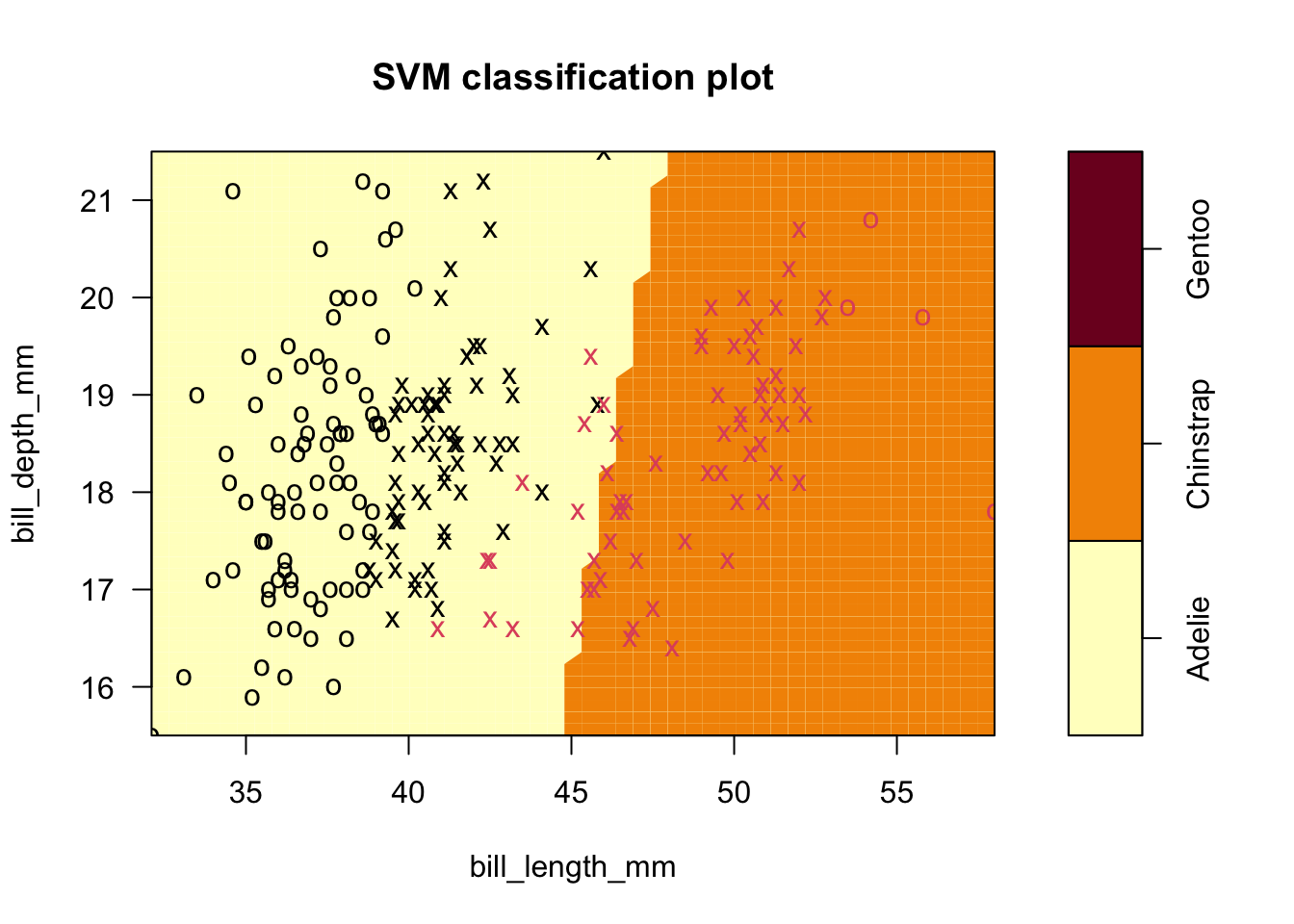
Code
summary(sv.fit.lin.lowCost)##
## Call:
## svm(formula = species ~ bill_length_mm + bill_depth_mm, data = penguins_1_2,
## kernel = "linear", cost = 0.01)
##
##
## Parameters:
## SVM-Type: C-classification
## SVM-Kernel: linear
## cost: 0.01
##
## Number of Support Vectors: 128
##
## ( 64 64 )
##
##
## Number of Classes: 2
##
## Levels:
## Adelie Chinstrap Gentoo5.4.3 Exercise 2
- The summary of the fit reveals 128 SVs were used, and you can see how the line shifted in an interesting manner.
- Now ten points are misclassified but they are all Chinstrap. It’s possible that some of the original support vector points were overly influential, but our approach has introduced more error.
5.5 The kernel trick
- The kernel trick is common to a great deal of machine learning techniques. It consists of two key ideas:
- Groups that are not linearly separable in \(p\) dimensions, may be separable in \(q\) dimensions, where \(q>p\), through a transformation.
- Rather than compute the transformation, train the model, and then predict on new data, we notice that a kernel function with a proper inner product generates an equivalent optimization problem and solution.
5.5.1 Illustration
- A rather extreme example of two circles makes the point. - Let one group be defined by the relationship: \(X_{1}^{2}+X_{2}^{2}={{1}^{2}}\) and the other by: \(X_{1}^{2}+X_{2}^{2}={{2}^{2}}\)
- If we transform the 2-D relationships to 3-D via the mapping: \(({{X}_{1}},{{X}_{2}})\mapsto ({{X}_{1}},{{X}_{2}},X_{1}^{2}+X_{2}^{2})\), we get clearly separable groups:
Code
set.seed(1001)
x1 <- runif(100,-2,2); y1 <- sqrt(4-x1^2)
x2 <- runif(100,-1,1); y2 <- sqrt(1-x2^2)
df <- data.frame(x1=c(x1,x1,x2,x2),x2=c(y1,-y1,y2,-y2))
df$z <- df$x1^2+df$x2^2
plot3D::scatter3D(df$x1,df$x2,df$z)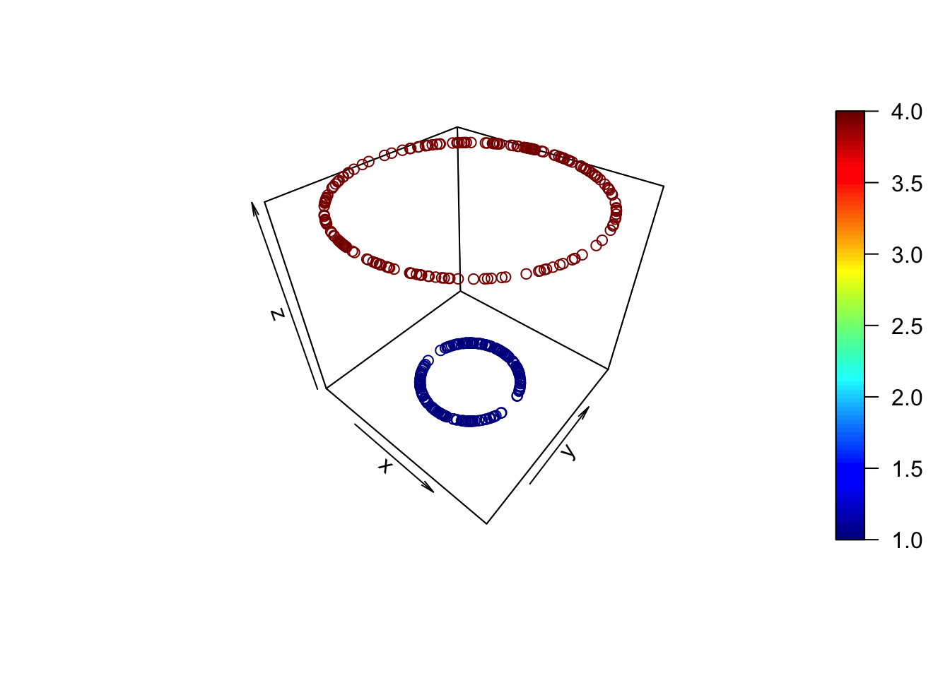
- Contrast the above to the 2-D original set of relationships:
Code
plot(x2~x1,data=df,col=c(4,2,2,3)[round(z)]) 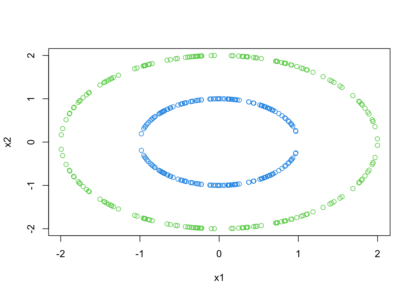
- Rather than transform/solve/train on training data and then transform/predict on new data, we note that training involved an inner product.
- To understand this, we have to reformulate the optimization problem using what is known as the ‘dual’. \(Let \ \vec{\beta} = \sum_{i=1}^{N}\alpha_iY_i\vec{X}_i\).
- The new, equivalent optimization problem is: We want
\[ \underset{{\vec{\alpha }}}{\mathop{\max }}\,\sum\limits_{i=1}^{N}{{{\alpha }_{i}}}-\frac{1}{2}\sum\limits_{i,j=1}^{N}{{{\alpha }_{i}}{{\alpha }_{j}}{{Y}_{i}}{{Y}_{j}}{{{{\vec{X}}'}}_{i}}}{{\vec{X}}_{j}} \] with constraints \(\sum\limits_{i=1}^{N}{{{\alpha }_{i}}{{Y}_{i}}}=0\) and \(\forall i=1,\ldots,N,\ \ 0\le {{\alpha }_{i}}\le C\).
- The vector notation is similar for
\[ \vec\alpha=[\alpha_1,\ldots ,\alpha_n]' \]
The term
\[ \left\langle{\vec{X}_i},\vec{X}_j \right\rangle = \vec{X}_i^{\prime}\vec{X}_j=\sum\limits_{k=1}^{p}X_{ki}X_{kj} \]
is an (linear) inner product capturing a pairwise relationship between two vectors, which are points in our feature space.
- Also,
\[ \left\langle {{{\vec{X}}}_{i}},{{{\vec{X}}}_{j}} \right\rangle =\left\| {{{\vec{X}}}_{i}} \right\|\left\| {{{\vec{X}}}_{j}} \right\|\cos (\theta ) \]
where \(\theta\) is the angle between the vectors and the norms are Euclidean (think distance from 0).
- So this is some measure of similarity (non-orthogonality).
- Some example vectors (points in 2-space) along with their inner product follows.
- Note that the extent to which the points (features) ‘agree’ on the two dimensions yields larger values of the measurement
- Opposite directions, or complete disagreement yields negative values.
Code
vs <- matrix(c(1,1,1,-1,-1,-1,-1,1,0,1.5),ncol=2,byrow=T)
plot(vs,ylim=c(-1.5,2),xlim=c(-2.5,2.5),pch=16,cex=2,col=2:7,xlab="X1",ylab="X2")
abline(v=0,col=8); abline(h=0,col=1,lwd=2)
ds <- vs%*%t(vs)
chs <- matrix(c(1,5,2,3,2,4),ncol=2,byrow=T)
dests <- cbind(ds[chs],0)
points(dests,pch=16,col=8,cex=2)
arrows(vs[t(chs),1],vs[t(chs),2],rep(dests[,1],each=2),rep(dests[,2],each=2),col=1+t(chs),length=.1)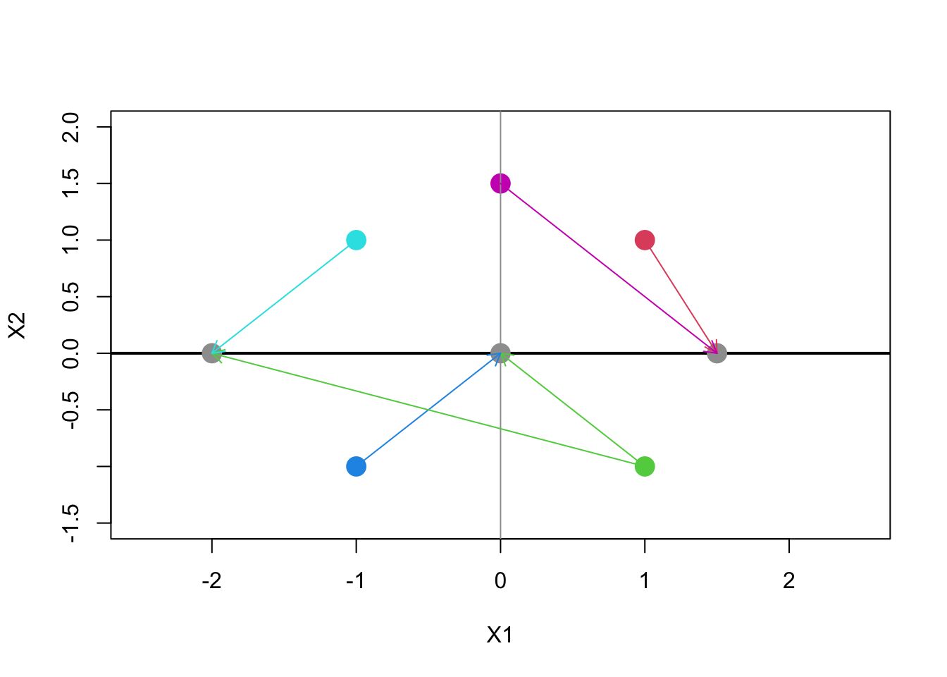
5.5.2 Exercise 3
- We rewrite the maximization problem in terms of the inner product, as follows:
\[ \underset{{\vec{\alpha }}}{\mathop{\max }}\,\sum\limits_{i=1}^{N}{{{\alpha }_{i}}}-\frac{1}{2}\sum\limits_{i,j=1}^{N}{{{\alpha }_{i}}{{\alpha }_{j}}{{Y}_{i}}{{Y}_{j}}K({{{\vec{X}}}_{i}},{{{\vec{X}}}_{j}})} \]
with
\[ K({{\vec{X}}_{i}},{{\vec{X}}_{j}})=\left\langle {{{\vec{X}}}_{i}},{{{\vec{X}}}_{j}} \right\rangle \]
and the same constraints as before.
- The first part of the kernel trick involves noting that inner product spaces are projections of higher dimensional spaces onto the real line, and that our groups may be separable in that higher dimensional space.
- The second part of the kernel trick involves noting that we only need the kernel function, \(K\), (not the projection onto a higher dimensional space) to solve the optimization problem.
- The ‘trick’ involves substituting a different kernel functions into the equations.
5.6 Kernel functions
- A frequently used kernel is the Gaussian, which can be parameterized in different ways.
- In R’s implementation, it is called the ‘radial’ kernel, defined as
\[ K(\vec{X}_i,\vec{X}_j) = \exp{\left(-\gamma{\left\| \vec{X}_i-\vec{X}_j\right\|}^2\right)} \]
- The inner term is the squared Euclidean distance between the two points.
- Open scaling parameter \(\gamma\) potentially yields a better classifier.
5.6.1 Application of svm to concentric circle data
Before going into details, we run svm on the circle data using several different kernels. First the linear:
Code
sv.circ.lin <- svm(factor(z)~ x1+x2,data = df, kernel='linear')
plot(sv.circ.lin,df,formula=x2~x1,main="Linear Kernel")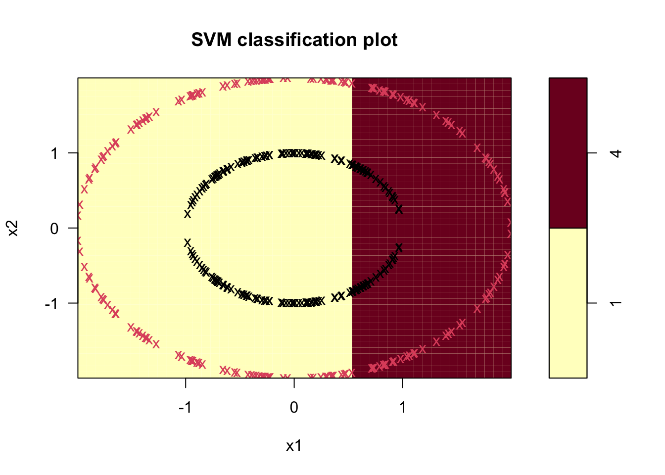
Using the Radial Kernel:
Code
sv.circ.rad <- svm(factor(z)~ x1+x2,data = df, kernel='radial')
plot(sv.circ.rad,df,formula=x2~x1)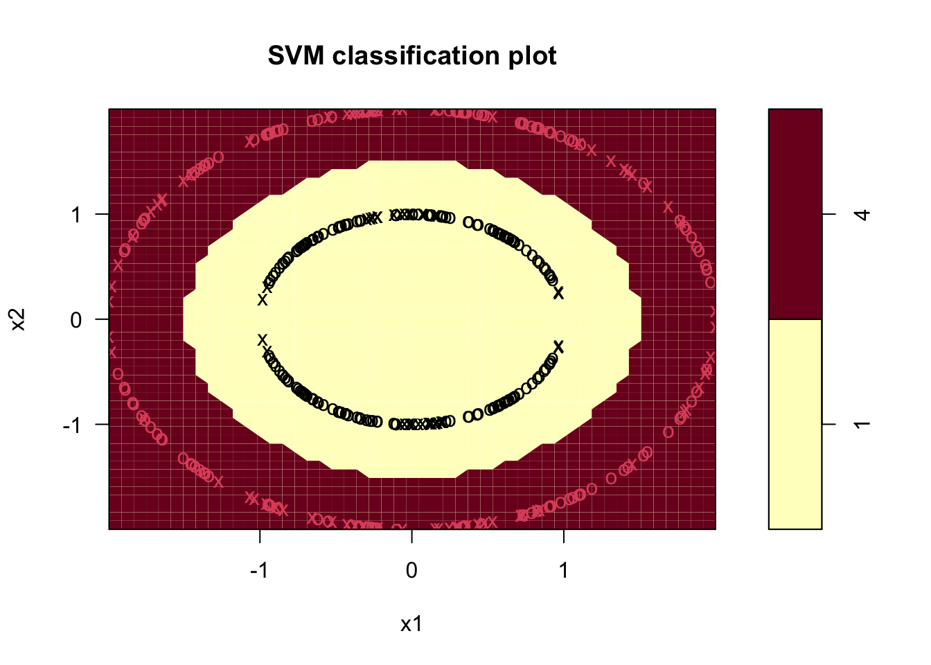
5.7 Examples of svm
- Alternative kernels and extensions to more than two groups.
- Extension of example two with radial kernel, default settings (\(C=1\), \(\gamma=0.5\)) for two-dimensional problems.
- PLOT ON NEXT PAGE.
- Note the curvature: this is what is a line (or plane) in the higher dimensional space looks like projected down onto the 2-space.
- We misclassify 7 observations. (exercise: carefully create the Confusion Matrix)
- Extension of example two with radial kernel, default settings (\(C=1\), \(\gamma=0.5\)) for two-dimensional problems.
5.7.1 Radial kernel
Code
sv.fit.rad <- svm(species ~ bill_length_mm+bill_depth_mm, data = penguins_1_2,kernel='radial')
plot(sv.fit.rad,penguins_1_2,formula=bill_depth_mm ~ bill_length_mm)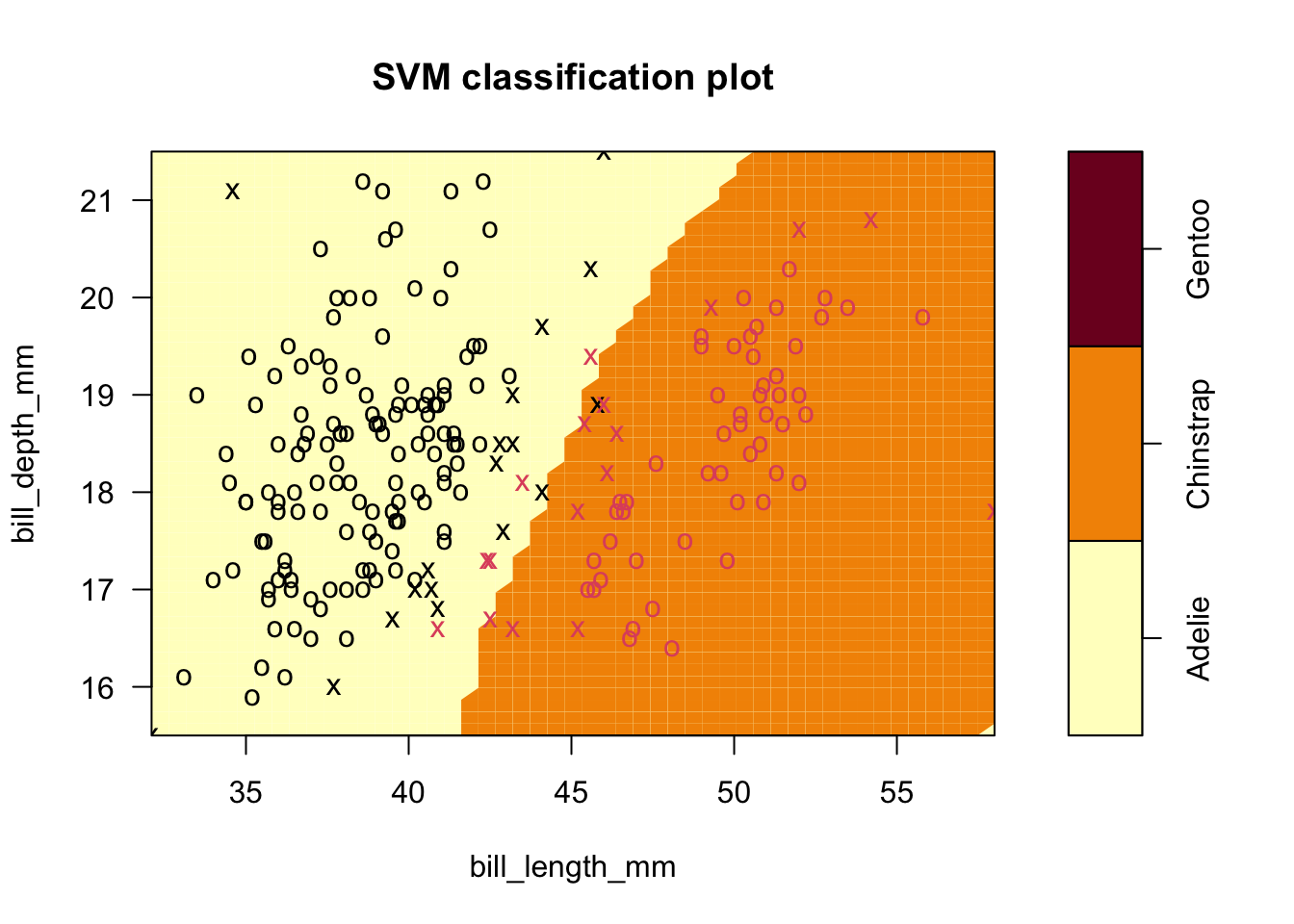
- We can change the parameters to improve classification
- We must be careful: to avoid overfitting, a method such as cross-validation (next Handouts) should be used to choose parameters.
- In this example, \(\gamma\) is increased to 2, which should exaggerate large differences between points.
- Only 5 observations are misclassified with these settings, as the boundary between groups is closed off around the Chinstrap.
Code
sv.fit.rad.gam2 <- svm(species ~ bill_length_mm+bill_depth_mm, data = penguins_1_2,kernel='radial',gamma=2)
plot(sv.fit.rad.gam2,penguins_1_2,formula=bill_depth_mm ~ bill_length_mm)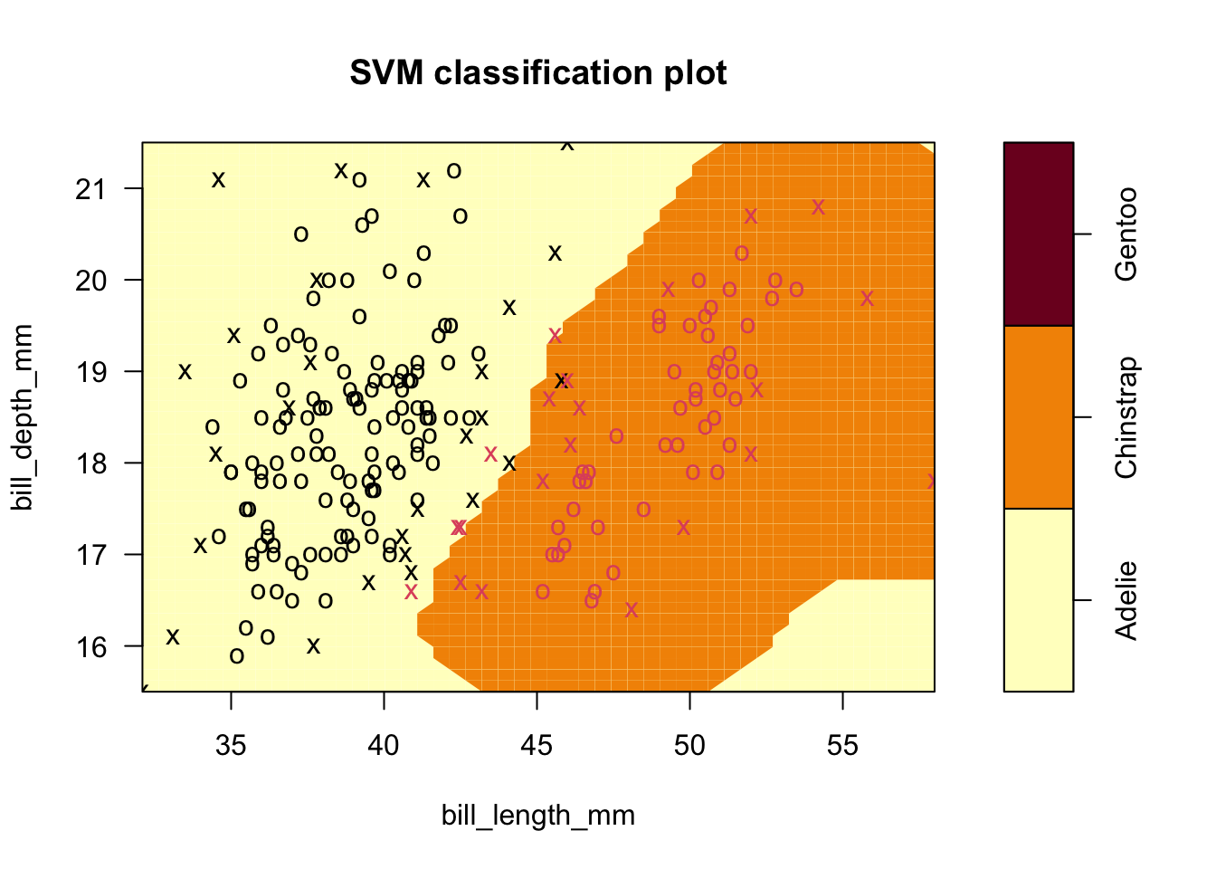
5.7.2 SVM with more than two groups.
- The basic idea is to do SVM recursively
- Group one vs. all else; group two vs. groups three and higher, etc.
- Example four: use all species in penguins data (finally!).
- Linear followed by radial kernel fits (default settings).
- Notice, as before, that it is easy to separate Gentoo from the rest.
- Also, we don’t gain predictive power from this extension
- It’s still hard to distinguish Adelie and Chinstrap at the boundary, and radial kernel only helps a little.
- Linear followed by radial kernel fits (default settings).
Code
sv.fit.lin_all3 <- svm(species ~ bill_length_mm+bill_depth_mm, data = penguins,kernel='linear')
plot(sv.fit.lin_all3,penguins,formula=bill_depth_mm ~ bill_length_mm)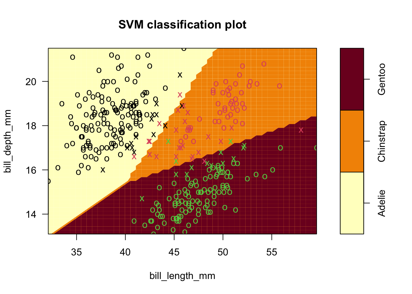
Code
#caret::confusionMatrix(sv.fit.lin_all3$fitted,penguins$species)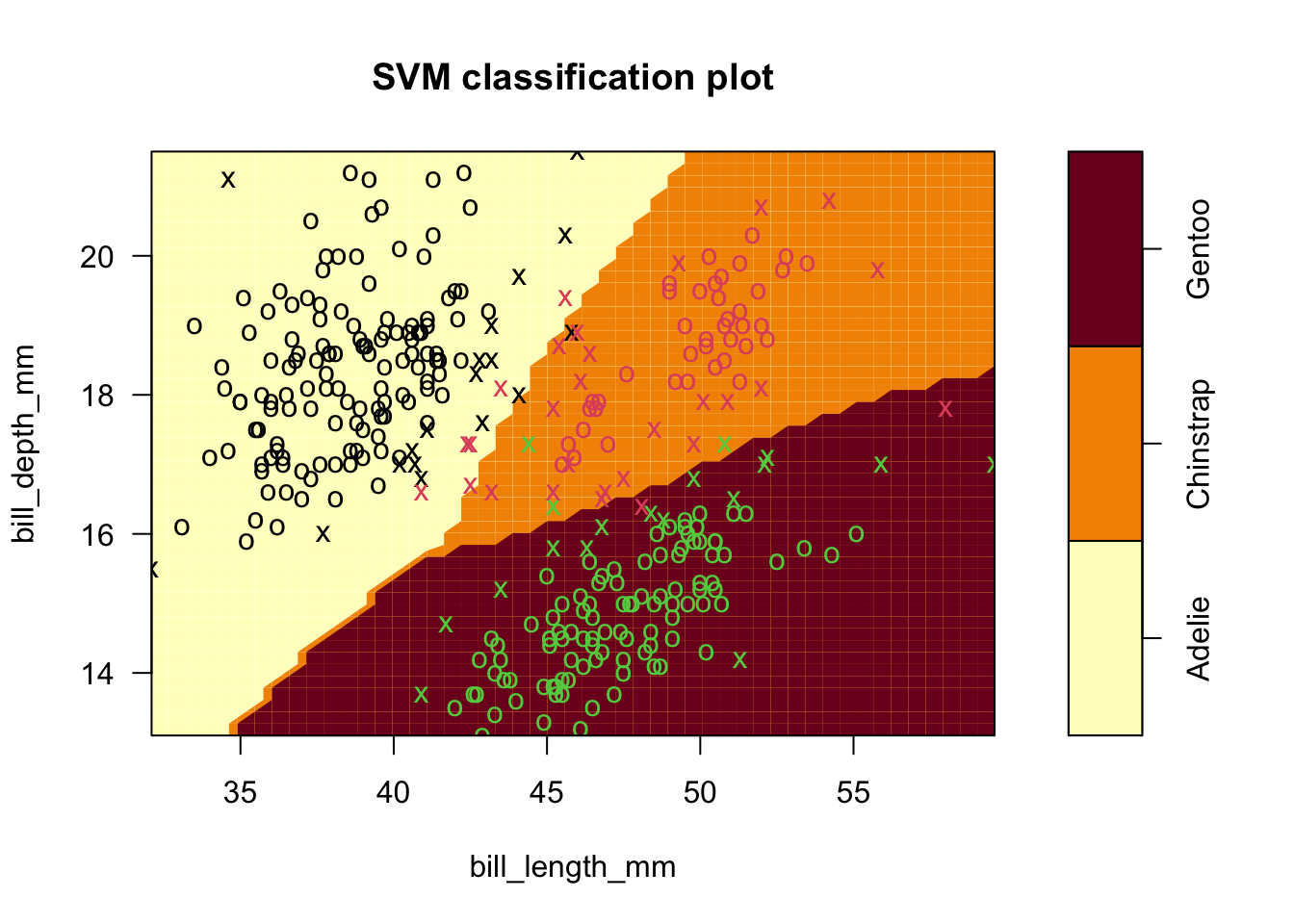
5.8 Cross-validation
- The basic idea is to withhold a sample of your training data as test data
- First, loop through any open parameters (e.g., \(C\), \(\gamma\)) and ‘fit’ with those held constant on the training set
- Evaluate performance on the test set.
- Do this repeatedly and then pick the best parameters.
- Evaluate performance on the test set.
- First, loop through any open parameters (e.g., \(C\), \(\gamma\)) and ‘fit’ with those held constant on the training set
- We did this for penguins data, still trying to classify using only two features (petal measurements)
- Used a ‘grid search’ of \(C=0.01,0.1,1,10,100\), and \(\gamma\)=0.5,1,2,3,4)
- Surprisingly, the best parameters are the defaults in this case!
Code
set.seed(1001)
tune.out <- tune(svm, species ~., data=penguins, kernel='radial', ranges = list(cost=c(0.01,0.1,1,10,100),gamma=c(0.5,1,2,3,4)))
summary(tune.out)
##
## Parameter tuning of 'svm':
##
## - sampling method: 10-fold cross validation
##
## - best parameters:
## cost gamma
## 1 0.5
##
## - best performance: 0.01194296
##
## - Detailed performance results:
## cost gamma error dispersion
## 1 1e-02 0.5 0.56140820 0.07637943
## 2 1e-01 0.5 0.02994652 0.02426397
## 3 1e+00 0.5 0.01194296 0.01542116
## 4 1e+01 0.5 0.01800357 0.01549880
## 5 1e+02 0.5 0.01800357 0.01549880
## 6 1e-02 1.0 0.56140820 0.07637943
## 7 1e-01 1.0 0.21301248 0.06868594
## 8 1e+00 1.0 0.01800357 0.01549880
## 9 1e+01 1.0 0.01800357 0.01549880
## 10 1e+02 1.0 0.01800357 0.01549880
## 11 1e-02 2.0 0.56140820 0.07637943
## 12 1e-01 2.0 0.54055258 0.07215674
## 13 1e+00 2.0 0.04803922 0.03230884
## 14 1e+01 2.0 0.03903743 0.02867112
## 15 1e+02 2.0 0.03903743 0.02867112
## 16 1e-02 3.0 0.56140820 0.07637943
## 17 1e-01 3.0 0.56140820 0.07637943
## 18 1e+00 3.0 0.08707665 0.04562229
## 19 1e+01 3.0 0.08110517 0.04697382
## 20 1e+02 3.0 0.08110517 0.04697382
## 21 1e-02 4.0 0.56140820 0.07637943
## 22 1e-01 4.0 0.56140820 0.07637943
## 23 1e+00 4.0 0.13493761 0.06282590
## 24 1e+01 4.0 0.12584670 0.06348637
## 25 1e+02 4.0 0.12584670 0.06348637Code
sv.fit.rad_all3 <- svm(species ~ bill_length_mm+bill_depth_mm, data = penguins,kernel='radial',cost=1,gamma=.5)
plot(sv.fit.rad_all3,penguins,formula=bill_depth_mm ~ bill_length_mm)
5.8.1 Exercise 5
- Dispersion, above, is like an RMSE (\(rmse=\sqrt{\frac{1}{n}\sum\limits_{i}{{{({{{\hat{y}}}_{i}}-{{y}_{i}})}^{2}}}}\)) measure and we want to minimize it.
- It is possible to set parameters to achieve better within-sample performance that does not translate to out-of-sample performance.