6 Chapter 6: Feature Sets, L.O.O., C.A.R.T., C.V., N.B.

Image source

6.1 LOO, Regression Tree (CART), Naive Bayers

• As suggested in class discussion last time, classification is a form of model building, and as such, one should explore more complex feature sets including polynomial terms and interactions.
  

• Example: penguins

• The potential for more complex features derived from the three measurements is large:

  • Squared terms
  • Ratios
  • Products (interactions).
    
  • These represent different measurements, such as area and shape.

• We explored all two-way interactions and then we added the body_mass_g variable that we have excluded up until now.

Code

require(MASS)
#Alt approach to classif - improve the feature set.
penguins$BL.BD <- penguins$bill_length_mm*penguins$bill_depth_mm
penguins$BL.FL <- penguins$bill_length_mm*penguins$flipper_length_mm
penguins$BD.FL <- penguins$bill_depth_mm*penguins$flipper_length_mm
penguins$Sp <- factor(c("a","c","g")[penguins$species]) #simpler label for plots.

6.1.1 Exercise 1

Question link

• We tried two different models (feature sets) and ran an LDA for each. The models are:
  1. ‘main effects’
  2. 1 plus all two-way interactions.
• The results are given next (think of the lines you would draw to separate the groups):

Code

penguins.lda.5 <- lda(Sp~bill_length_mm+bill_depth_mm+flipper_length_mm, data=penguins)
plot(penguins.lda.5,col=(2:4)[penguins$species])

Code

penguins.lda.int1 <- lda(Sp~bill_length_mm+bill_depth_mm+flipper_length_mm+BL.BD+BL.FL+BD.FL, data=penguins)
plot(penguins.lda.int1,col=(2:4)[penguins$species])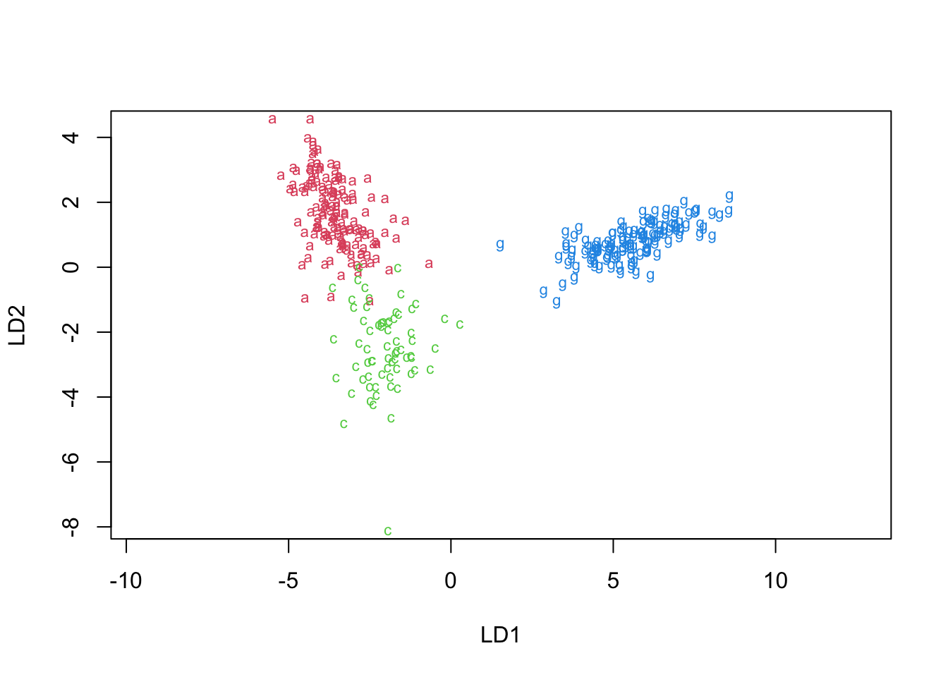

Code

penguins.lda.int1plus <- lda(Sp~bill_length_mm+bill_depth_mm+flipper_length_mm+BL.BD+BL.FL+BD.FL+body_mass_g, data=penguins)
plot(penguins.lda.int1plus,col=(2:4)[penguins$species])

2. The classification tables look like this (in order 1-3):

Code

xtabs(~penguins$species+predict(penguins.lda.5,penguins)$class)

##                 predict(penguins.lda.5, penguins)$class
## penguins$species   a   c   g
##        Adelie    145   1   0
##        Chinstrap   5  63   0
##        Gentoo      0   0 119

Code

xtabs(~penguins$species+predict(penguins.lda.int1,penguins)$class)

##                 predict(penguins.lda.int1, penguins)$class
## penguins$species   a   c   g
##        Adelie    144   2   0
##        Chinstrap   4  64   0
##        Gentoo      0   0 119

Code

xtabs(~penguins$species+predict(penguins.lda.int1plus,penguins)$class)

##                 predict(penguins.lda.int1plus, penguins)$class
## penguins$species   a   c   g
##        Adelie    144   2   0
##        Chinstrap   3  65   0
##        Gentoo      0   0 119

• Models 1 & 2 have 6 errors, but they are quite different
  • We have achieved one fewer error in the last LDA ‘model’
  • We might be able to use different types of interactions to improve the model further.
  • While this is an achievement, what might we expect from a new sample of penguins?

6.2 Leave One Out Cross-Validation (L.O.O.)

• If one is primarily interested in describing which features best discriminate groups, then LDA using all of the data can be gainfully employed.
• If one expects to use the discriminant functions (projections) to classify new data, then the above ‘success’ rate is likely to be overly optimistic.
• One way to get a more realistic assessment of the likely ‘out of sample’ success rate involves the L.O.O. strategy:
  • If there are N data points, plan to fit the LDA model N times.
  • On iteration \(i\), leave out the \(i^{th}\) observation, fit the model, and then predict the ith observation with that model.
    • Since the ith observation was excluded during the model-building (training) phase, it can have no influence on the model itself.
  • Report the average classification success rate based on these predictions.
  • LDA (in MASS R library) does this for you (CV=TRUE option).

6.2.1 LOO using the penguins data

Code

penguins.lda.5Loo <- lda(Sp~bill_length_mm+bill_depth_mm+flipper_length_mm, data=penguins,CV=T)
penguins.lda.int1Loo <- lda(Sp~bill_length_mm+bill_depth_mm+flipper_length_mm+BL.BD+BL.FL+BD.FL, data=penguins,CV=T)
penguins.lda.int1plusLoo <- lda(Sp~bill_length_mm+bill_depth_mm+flipper_length_mm+BL.BD+BL.FL+BD.FL+body_mass_g, data=penguins,CV=T)

xtabs(~penguins$species+penguins.lda.5Loo$class)

##                 penguins.lda.5Loo$class
## penguins$species   a   c   g
##        Adelie    145   1   0
##        Chinstrap   5  63   0
##        Gentoo      0   0 119

Code

xtabs(~penguins$species+penguins.lda.int1Loo$class)

##                 penguins.lda.int1Loo$class
## penguins$species   a   c   g
##        Adelie    143   3   0
##        Chinstrap   4  64   0
##        Gentoo      0   0 119

Code

xtabs(~penguins$species+penguins.lda.int1plusLoo$class)

##                 penguins.lda.int1plusLoo$class
## penguins$species   a   c   g
##        Adelie    144   2   0
##        Chinstrap   3  65   0
##        Gentoo      0   0 119

6.2.2 Exercise 2

Question link

6.2.3 Notes

• We make 5,6, or 7 errors depending on which model is chosen
• PLOTTING: hard to plot the predictions (projections) made under the LOO strategy
  • While most software reports the classification based on LOO, you have to check carefully as to whether the software will provide the projected point in the LDA space.
• As a first pass, we projected the points using the full training set (non-LOO) and our most complex model (3).
  • This is the wrong predictive model (never changes), so it is problematic.

Code

#harder to plot (use non-LOO version for LD1,2):
locs <- predict(penguins.lda.int1plus,data.frame(penguins[,c(3:5,9:11,6,12)]))$x
plot(locs,col=c(3,2,4)[penguins$Sp],pch=c("a","c","g")[penguins$Sp])
bb <- penguins$Sp != penguins.lda.int1plusLoo$class
points(locs[bb,],pch=1,col=c(3,2,4)[penguins.lda.int1plusLoo$class[bb]],cex=1.8)

6.2.4 Exercise 3

Question link

6.3 Classification & Regression Trees (CART)

• Motivation: use a set of ‘decision rules’ to classify observations based on a feature set.
• With the penguins data, e.g., it was clear that we could ‘split off’ the Gentoo species from the rest by many of the features, the combination of bill depth and flipper length was apparent.
• Can we take this idea further, separating species by a series of decision rules about the features?
• CART is a method that formalizes the simple idea that if you choose the right set of YES or NO questions, you can classify or identify membership.
  • E.g., the game ‘20 Questions’ allows one to ask a series of YES/NO questions that inform the player as to the likely ‘secret object.’
  • More formally, the underlying structure is known as a binary tree, as there are two branches off of any node (question).
  • One moves down a binary tree accumulating ‘YES/NOs’ or True/Falses, or even ‘-’ and ‘.’ (i.e., Morse code).

6.3.1 Known CART example

• What if we start with two features from the penguins data and try to build a series of questions to classify the species.
  • Let’s first remind ourselves of how separated the species are by examining a ‘pairs’ plot.
  • Are there two features that separate species well?
    
  • Can we build a set of binary questions for that purpose?

6.3.2 Pairs plot

Code

#reminder of the penguins Data separation into Species:
pairs(penguins[,3:5],col=c(3,2,4)[penguins$species],pch=as.character(penguins$species))

6.3.3 Formal approach to building CART ‘prediction models’

• Select a set of question ‘types’ to ask.
  • Usually, these are of the form: ‘is the value of this feature less than a specific value?’ or for categorical features, it might be, ‘is the value of this feature in a specific set (e.g., colors red and orange)?’
• Choose a mechanism to decide between questions
  • An objective function that ranks each potential split as ‘better’ or ‘worse’ than the others.
• Choose a stopping rule (otherwise, one could keep splitting nodes until only a single observation was left).
• Have a way to classify observations at any node (usually majority rules).

6.3.4 Rpart

• The R function, rpart, recursively partitions the data using simple cutoffs for continuous predictors, and builds a decision tree in the process.
  • The user specifies the feature set to explore using an R ‘formula’ (looks a bit like a prediction equation without coefficients).
  • The user can specify the minimum size a node must be in order to be eligible to be split.
  • The user specifies a stopping criterion (default is less than 1% improvement in classification rate).
  • The user can define a criteria for selecting optimal cut points, but the two choices, ‘gini’ and ‘information’ have similar results in our data, so we stick to information, which involves the entropy of the split.
    • Entropy reflects disorder, or uncertainty of classification. The highest entropy exists when there are N categories, and the objects are distributed equally among them. Lowest is when all objects are concentrated in ONE category.

6.3.5 CART example using rpart and the penguins data.

• We will specify the relationship between Species and the original feature set (3 measures)
  • Allow splits of nodes up to size 2 (really, this is not a restriction)
  • Use the default criterion of percent change in classification must be > 1%, or the algorithm will ‘stop’.

Code

library(rpart)
#reminder: Sp is a recoded factor of the 3 species.
fit1 <- rpart(species~bill_length_mm+bill_depth_mm+flipper_length_mm, control=rpart.control( minsplit=2), data=penguins)

6.3.6 Graphical display of results (rpart.plot functions)

Code

rpart.plot(fit1)

6.3.7 Exercise: walk through classification of first penguin in the dataset

Code

pred1 <- predict(fit1,type='class')
confusionMatrix(pred1, penguins$species)$table

##            Reference
## Prediction  Adelie Chinstrap Gentoo
##   Adelie       142         1      0
##   Chinstrap      4        67      1
##   Gentoo         0         0    118

• You can see how the ‘majority rules’ classification works (look at the bottom nodes).
  
• You can see how a simple set of questions leads to ‘only’ 6 missclassifications.
  • Fine point: the ‘extremes’ one might have to go to in order to get some of the smaller nodes correct might not be worth it, as we’d be ‘overtraining’.
    
  • There is a notion of ‘pruning’ the tree that would remove such overfitting anyway.

6.3.8 Visualization (splits as binning)

• To understand recursive partitioning as a form of splitting and binning, we refit the penguins data using only two features, bill and flipper length
• Using a library only available on Git, we shade the space of predictions using colors that map to the three species.
  • Shades in each partition indicate the overarching classification in that section.
• There are more classification errors with this approach, but it illustrates the rpart concept in 2D.

Code

fit2 <- rpart(species~bill_length_mm+flipper_length_mm, control=rpart.control( minsplit=2), data=penguins)
pred2 <- predict(fit2,type="class")

Code

gg<-ggplot(data=penguins,aes(y=bill_length_mm,x=flipper_length_mm,color=species))+geom_text(aes(label=Sp),hjust=0.5, vjust=0.5)+geom_parttree(data = fit2, aes(fill=species), alpha = 0.1)+theme(legend.position = "none")
gg

## Warning: Using the `size` aesthetic in this geom was deprecated in ggplot2 3.4.0.
## ℹ Please use `linewidth` in the `default_aes` field and elsewhere instead.

• The correct classification is given by the letter.
  • Fine point: the simple partitioning does not allow for non-vertical or horizontal cuts. Linear models (e.g., LDA, regression), do allow for this type of cut.
    • Thus CART, tends to do well when there are non-linear relationships between features and response.
      
    • It’s a non-parametric method, as well.

6.4 Cross-validation: introduction & sketch

• One of the criticisms of CART and many classification techniques is that they overfit the data, meaning they use ALL of the data when building a model, so they may pick up idiosyncrasies specific to this data and when new data arrive, they will be poor classifiers.
• One approach to dealing with this is to train the classifier on a subset of data and then test it on a remaining sample.
  • This is called cross-validation (CV)
  • This is also useful in SEM, factor analysis, regression, etc.

6.4.1 K-folds

• A K-folds approach to CV is to partition the data into K equal portions.
  • Withhold each portion ONCE; fit the classification model on the remaining (training) data and CLASSIFY on the withheld portion.
  • Assess the classification (% correct)
  • Repeat for each of the K folds; take the average success rate as the benchmark of what to expect in new samples.
  • The random partitioning can be repeated to ensure that the K-folds themselves were not idiosyncratic.
• Do you expect the CV benchmarked classification rate to be higher or lower than that based on the full sample (in which training and test data are identical)?

6.4.2 Cross Validation with CART

• There are packages to make CV ‘easier’ but with rpart, I found it easier to write my own routine to do the CV.
• Below, I reproduce the code, and then describe it briefly.

Code

#set up for cv:
corr.rate.sum <- 0
R <-10
K <- 10
len <- dim(penguins)[1] #number of obs
set.seed(2011)
#penguins is of size 333 - need to handle non-mult of 10
remainder  <- len - K*floor(len/K)
fit.cv <- vector("list",K)
for (i in 1:R) {
  idx <- sample(c(1:remainder,rep(1:K,each=floor(len/K))),replace=F)
  corr.sum <- 0 
  for (j in 1:K) {
    fit.cv[[j]] <- rpart(species~bill_length_mm+bill_depth_mm+flipper_length_mm,  control=rpart.control(minsplit=2), parms=list(split="information"), data=penguins[idx!=j,])
    preds <- predict(fit.cv[[j]],penguins[idx==j,],type="class")
    corr.ct <- sum(preds==penguins$species[idx==j])
    corr.sum <- corr.sum + corr.ct    
  }
  corr.rate.sum <- corr.rate.sum + corr.sum/len
}
cat('overall K=',K,'fold, R=',R,'repeat success rate:',corr.rate.sum/R,'\n')

## overall K= 10 fold, R= 10 repeat success rate: 0.9504505

6.4.3 Code description

• ‘R’ is number of repeats; ‘K’ is the number of folds associated with each repeat.
• The numbers 1-K are repeated over and over so that the same number of \(1,2,\ldots K\) are in each sample (and these numbers are shuffled).
  • These are the indices of the ‘leave out’ sample.
    
  • If K=4, you can think of cards in a deck, and you leave out one ‘suit’ each time you fit the model and evaluate on test data.
• An rpart fit is made to the training sample and then a prediction is made on the test sample (the left out ‘fold’ or suit).
• The number correctly classified is tallied.
• The process is repeated for each fold, tallied, and accumulated for an overall average success rate.

6.4.4 Last tree corresponding to ‘folds’ 1-9 of the data

• They are often quite similar, if you look closely
• They have been trained on a subset of the data, so should not be as accurate as if they were trained on all of it.
• The advantage to this is that it sets expectations closer to what would happen in practice when you receive new data.
• A success rate of 95%, which is a bit higher than the non-CV approach, but reflects expectations from future samples.
• In ‘big data’ problems, the ‘LOO’ strategy of leaving out only ONE point at time is not practical, computationally.
  • 10 folds (a 90% training, 10% test sample) is commonly used.

6.4.5 Ways to improve CART

1. Bagging
2. Boosting
3. Random Forests
4. Go Bayesian: BART

6.5 Naïve Bayes classifier

• Some intuition as to how prediction engines work (in general) can be gained by examining the Naïve Bayes Classifier.
• Bayes’ Rule: this simple rule lies at the heart of many prediction models & algorithms, because it allows one to ‘invert’ a problem as follows:
  • Say there are two events, A & B. Then Bayes’ Rule is simply: \(P(A|B)=\frac{P(B|A)P(A)}{P(B)}\).
    
  • It is precisely the definition of conditional probability, once we realize that the numerator is \(P(AB)=P(B|A)P(A)\).
• Typically, A takes on discrete values \(1,\ldots, J\), and B is a little more complex; namely, \(B={X_1,X_2,\ldots,X_P}\) is a feature set (the training data features).
• Restating A & B as terms in a classification problem, we are given training data (features) \(X_1,X_2,\ldots,X_P\) for records \(i=1,\ldots,N\), and N corresponding labels (groups), \({{A}_{i}}\in \{1,\ldots ,J\}\).
• Our goal is to predict the label (group) for a new observation given features \(X_1,X_2,\ldots,X_P\).

6.5.1 Extending Bayes’ Rule

\[ P(A|{{X}_{1}},\ldots ,{{X}_{P}})=\frac{P({{X}_{1}},\ldots ,{{X}_{P}}|A)P(A)}{P({{X}_{1}},\ldots ,{{X}_{P}})} \]

• The denominator acts as a constant in this problem, and simply insures that the left hand side is a probability (between 0-1 and sum over all events A is 1).
  
• The term P(A) is the prior distribution of A
  • i.e., our prior beliefs about A, which in the case of classification will be discrete.
• Interest (and challenge!) lies in estimating \(P({{X}_{1}},\ldots ,{{X}_{P}}|A)\) from the data.
  • This is a very high dimensional density estimation problem (hard: think- as hard as estimating covariance matrices).
  • Note: we need \(P({{X}_{1}},\ldots ,{{X}_{P}}|A)\), the probability of the data given the discrete class A, because it directly relates to the probability of a discrete class in A given the data \(X_1,X_2,\ldots,X_P\).

6.5.2 Key insight/idea

• Replace the multivariate density with a product of univariate densities.
  • This is called the NB assumption; that given the class A, realizations of \(X_k\) are independent, for \(k=1,\ldots,P\) (conditional independence assumption)
    • This yields the Naïve Bayes classification rule: Namely, we assume: \(P({{X}_{1}},\ldots ,{{X}_{P}}|A)=\prod\nolimits_{k=1}^{P}{P({{X}_{k}}|A)}\).
      
    • The terms inside the product are often estimated using kernel density estimators when continuous, or simply empirical distribution functions when discrete.

6.5.3 Notes

• Conditional Independence is actually a very strong assumption, as it suggests that complex multivariate dependencies can be replaced by marginal (indep.) products.
  • But it tends to work very well in practice.
• With this simplification, we can separate the data by the discrete labels \(A=1,\ldots,J\), and then estimate each \(P({{X}_{k}}|A)\) separately, combining them as \(\prod\nolimits_{k=1}^{P}{P({{X}_{k}}|A)}\).
• Once trained, for a new observation, \(A^{*}\)and features \(X_{1}^{*},\ldots ,X_{P}^{*}\), we can compare \(\prod\nolimits_{k=1}^{P}{P(X_{k}^{*}|{{A}^{*}}}=j)\), for \(j=1,\ldots,J\) and choose the \(j\) that maximizes that expression.
• Another way to write this, if we call the target label \(Y\), is: \({{Y}_{pred}}\leftarrow \arg {{\max }_{j}}P(Y=j)\prod\limits_{k}{(P({{X}_{k}}}|Y=j)\) for feature set \(X_{1}^{{}},\ldots ,X_{P}^{{}}\)

6.5.4 Example using the penguins data, in R, with 90/10 folded cross validation (and caret package):

Code

x <- model.matrix(~-1+bill_length_mm+bill_depth_mm+flipper_length_mm,data=penguins)
y <- penguins$species
set.seed(2011)
fit2cv <- train(x,y,'nb',trControl=trainControl(method='cv',number=10))

## Warning in FUN(X[[i]], ...): Numerical 0 probability for all classes with
## observation 20

Code

print(fit2cv)

## Naive Bayes 
## 
## 333 samples
##   3 predictor
##   3 classes: 'Adelie', 'Chinstrap', 'Gentoo' 
## 
## No pre-processing
## Resampling: Cross-Validated (10 fold) 
## Summary of sample sizes: 299, 300, 300, 302, 299, 300, ... 
## Resampling results across tuning parameters:
## 
##   usekernel  Accuracy   Kappa    
##   FALSE      0.9698580  0.9524430
##    TRUE      0.9668277  0.9476811
## 
## Tuning parameter 'fL' was held constant at a value of 0
## Tuning
##  parameter 'adjust' was held constant at a value of 1
## Accuracy was used to select the optimal model using the largest value.
## The final values used for the model were fL = 0, usekernel = FALSE and adjust
##  = 1.

Code

post2cv<-predict(fit2cv$finalModel,x)$posterior

## Warning in FUN(X[[i]], ...): Numerical 0 probability for all classes with
## observation 179

Code

df <- data.frame(post2cv,TrueSpecies=penguins$species)
df <- reshape2::melt(df)

## Using TrueSpecies as id variables

Code

gg<-ggplot(df, aes(x=value, color=TrueSpecies)) + geom_histogram(fill="white", alpha=0.5, position="dodge") + labs(x='Prob(facet species)',y='Frequency') + facet_grid(variable~"Facet")

Code

gg

## `stat_bin()` using `bins = 30`. Pick better value with `binwidth`.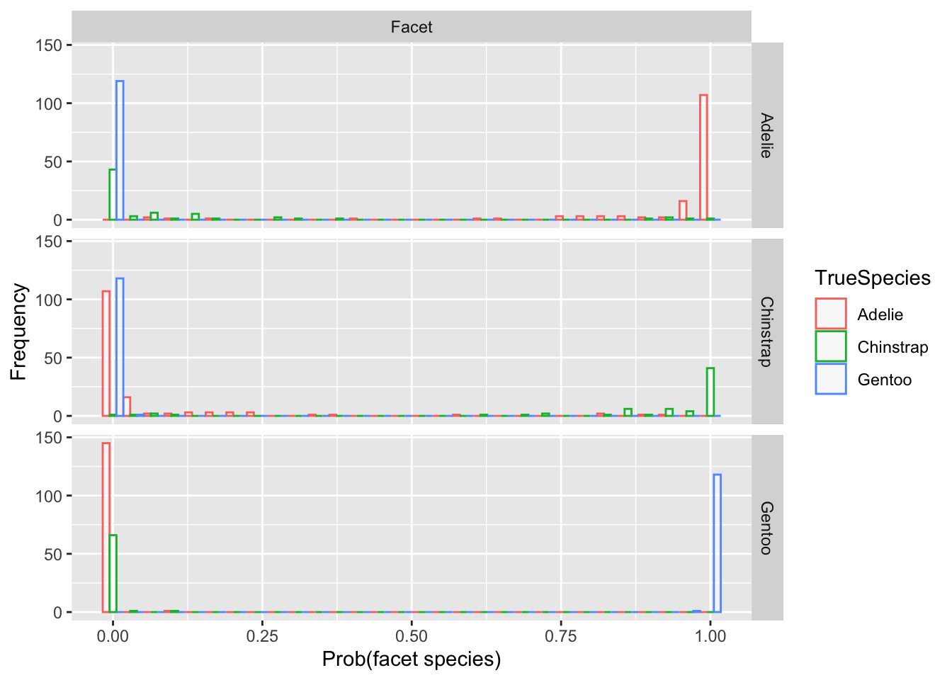

6.5.5 Notes

• The predictions near 0 or 1 are correct
  • In between is the area of ambiguity.
    
• As a direct by-product of the Naïve Bayes Classifier, the conditional densities of the features, given the label, are available (means and std. devs.):

Code

fit2cv$finalModel$tables

## $bill_length_mm
##               [,1]     [,2]
## Adelie    38.82397 2.662597
## Chinstrap 48.83382 3.339256
## Gentoo    47.56807 3.106116
## 
## $bill_depth_mm
##               [,1]     [,2]
## Adelie    18.34726 1.219338
## Chinstrap 18.42059 1.135395
## Gentoo    14.99664 0.985998
## 
## $flipper_length_mm
##               [,1]     [,2]
## Adelie    190.1027 6.521825
## Chinstrap 195.8235 7.131894
## Gentoo    217.2353 6.585431

6.5.6 Visualization of posterior (conditional) densities

Code

par(mfrow=c(2,2));  for (i in 1:3) { #inlining the code to save space
  plot(fit2cv$finalModel,vars=fit2cv$finalModel$varnames[i],legendplot = F)
  legend("topright",legend=unique(penguins$species),lty=1:3,col=2:4,cex=.75) }

6.5.7 Lessons Learned: applying Naïve Bayes to Crabs data

• First, crabs features are highly correlated even within crab species, so we are surely in strong violation of the NB assumption of conditional independence.
• Next, we applied NB naively, using the defaults.
  • These led to some warnings about observations with 0 predicted probability across all classes.
    
  • This can occur when ‘new’ data is outside the realm of the training data.
    
  • It is surprising this occurred, because are training and test data are the same in this example.
  • Nevertheless, the default settings assume normality, and this was questionable as well.
    
  • I eventually include Laplace corrections (this should take care of the 0 probabilities, but doesn’t quite) and use kernel density estimation, which does not assume normality. There are still some warning messages, but we display the results and discuss here.

Code

crabs <- read.dta("./Datasets/crabs.dta")
crabs$group <- factor(2*(crabs$sex=="Female")+(crabs$species=="Orange"))
fit<-NaiveBayes(group~FL+RW+CL+CW+BD,data=crabs,fL=10,usekernel=T)
preds <- predict(fit)
df <- data.frame(preds,Sex=crabs$sex,Species=crabs$sp)[,-1]
names(df)[1:4] <-c("Blue:Male","Orange:Male","Blue:Female","Orange:Female")
df <- melt(df)

## Using Sex, Species as id variables

Code

b <- apply(df[,c("Species","Sex")],1,paste,collapse=":")==df$variable
gg <- ggplot(df[b,], aes(x=value,color=variable))+scale_color_manual(values=c("darkblue","orange3","blue","orange1"))+geom_histogram(fill="white", alpha=0.5, position="dodge") + labs(x='Prob(Match Sex+Species)',y='Frequency') + facet_grid(Sex~Species)

Code

gg

## `stat_bin()` using `bins = 30`. Pick better value with `binwidth`.

6.5.8 Crosstab

Code

optLabel(preds$class,crabs$group)

## $match.by
## [1] "cols"
## 
## $best.match
## [1] 83
## 
## $best.perm
## [1] 1 2 3 4
## 
## $best.tbl
##    trg
## src  0  1  2  3
##   0  7  2  0  0
##   1  1  5  0  0
##   2 28 25 39 18
##   3 14 18 11 32

6.5.9 Terrible!

• The only successes are above 50%! (Almost always females)
  • What went wrong???
• What if we try to undo the correlation of the feature set?
  • We can try to do this using PCA.
    
• It turns out that this works very well, as the following run shows:

Code

crabs.comp <-princomp(crabs[,4:8],cor=F)$scores #not stdzd
crabs.pc <-crabs
crabs.pc[,4:8] <- crabs.comp
fit<-NaiveBayes(group~FL+RW+CL+CW+BD,data=crabs.pc,fL=10,usekernel=T)
preds <- predict(fit)
df <- data.frame(preds,Sex=crabs$sex,Species=crabs$sp)[,-1]
names(df)[1:4] <-c("Blue:Male","Orange:Male","Blue:Female","Orange:Female")
df <- melt(df)

## Using Sex, Species as id variables

Code

b <- apply(df[,c("Species","Sex")],1,paste,collapse=":")==df$variable
gg <- ggplot(df[b,], aes(x=value,color=variable))+scale_color_manual(values=c("darkblue","orange3","blue","orange1"))+geom_histogram(fill="white", alpha=0.5, position="dodge") + labs(x='Prob(Match Sex+Species)',y='Frequency') + facet_grid(Sex~Species)

6.5.10 Crabs Predicted Probabilities plot

Code

gg

## `stat_bin()` using `bins = 30`. Pick better value with `binwidth`.

6.5.11 Crosstab

Code

optLabel(preds$class,crabs$group) 

## $match.by
## [1] "cols"
## 
## $best.match
## [1] 191
## 
## $best.perm
## [1] 1 2 3 4
## 
## $best.tbl
##    trg
## src  0  1  2  3
##   0 46  0  2  0
##   1  1 50  1  2
##   2  3  0 47  0
##   3  0  0  0 48

6.5.12 Notes

• Classification rate of over 95%.

  • Sure, we should use CV to gauge better, but this is a vast improvement.
  • The classification probabilities are equally improved, as the final plot reveals.

• Methods like NB are powerful, when proper attention to the underlying assumptions is given.

• It’s a bit more work to visualize the classification errors, but one way is to plot the classification probabilities for each subject and each species.
  

• A good classifier will put nearly 100% of the probability on a single label (and mostly the correct one!)

• We ‘overfit’ the penguins data (do not use c.v.) and report the three posterior probabilities of each species graphically.

6.6 Lab

• Lab 6 link

6.7 Appendix

6.7.1 Introduction

• In this chapter, we will use supervised learning methods to classify diabetes from Diabetes Health Indicators Dataset. The dataset is a subset of The Behavioral Risk Factor Surveillance System (BRFSS) dataset, which is a health-related telephone survey that is collected annually by the Centers for Disease Control and Prevention (CDC).

• The target variable is Diabetes which has 2 classes - 0 is for no diabetes and 1 is for diabetes.

• Data that we use can be downloaded from this link.

• Following research paper used the dataset from the BRFSS.

  • Building Risk Prediction Models for Type 2 Diabetes Using Machine Learning Techniques

6.7.2 Application of models

• First, lets explore the dataset; we randomly subset the original dataset to increase model computation.

Code

library(ggplot2)
library(tidyverse)
library(ggrepel)
library(ROCR)
library(pROC)
library(e1071)
library(randomForest)
set.seed(2023)
df_ch6 <- read.csv("./Datasets/diabetes_data.csv") %>%
  sample_n(., 2000) %>%
  mutate(Diabetes = as.factor(Diabetes))
head(df_ch6)

##   Age Sex HighChol CholCheck BMI Smoker HeartDiseaseorAttack PhysActivity
## 1   7   1        1         1  40      0                    0            1
## 2   2   0        0         1  28      0                    0            1
## 3   8   1        0         1  30      1                    0            1
## 4  13   0        1         0  23      0                    0            1
## 5  13   0        0         1  28      0                    0            1
## 6   8   0        0         1  19      1                    0            0
##   Fruits Veggies HvyAlcoholConsump GenHlth MentHlth PhysHlth DiffWalk Stroke
## 1      1       1                 0       1        0        0        0      0
## 2      1       0                 0       1        0        0        0      0
## 3      1       1                 0       2       10        0        0      0
## 4      0       1                 0       2        0        0        0      0
## 5      1       1                 0       1        0        0        0      0
## 6      0       0                 0       2        0        0        0      0
##   HighBP Diabetes
## 1      1        0
## 2      0        0
## 3      0        0
## 4      1        1
## 5      1        0
## 6      0        0

• Next step is to divide the dataset into two parts: training and testing with certain ratio.

Code

# randomly splitting data with 7 to 3 ratio
train_ind <- sample(seq_len(nrow(df_ch6)), 
                    size = floor(0.7*nrow(df_ch6)))
train <- df_ch6[train_ind, ]
test <- df_ch6[-train_ind, ]

• Now, lets set up all the models that we want to use.

Code

# Support vector machines
# 1. linear
svm_linear_model<- e1071::svm(Diabetes ~ Age+Sex+HighChol+BMI+ Smoker+HeartDiseaseorAttack + PhysActivity + Stroke + HighBP,
                        data = train, 
                        kernel='linear')
svm_linear_pred = predict(svm_linear_model, newdata = test[-18])
# 2. radial
svm_radial_model<- e1071::svm(Diabetes ~ Age+Sex+HighChol+BMI+ Smoker+HeartDiseaseorAttack + PhysActivity + Stroke + HighBP,
                        data = train, 
                        kernel='radial')
svm_radial_pred= predict(svm_radial_model, newdata = test[-18])

# random forest
rf_model = randomForest(x = train[-18], y = as.factor(train$Diabetes) )
rf_pred = predict(rf_model, newdata = test[-18])

# Naive Bayers
nb_model = train( x=train[-18], y=train$Diabetes, method='nb')
nb_pred <- predict(nb_model, newdata = (test[-18]) )

• We use the same helper function from chapter 4 with a little modification.

Code

check_perf <- function(model,type){
  if (type=="unsuper"){
  acc <- confusionMatrix(data=model, 
                reference=factor(as.numeric(test$Diabetes)))$overall[[1]]    
  } else{
  acc <- confusionMatrix(data=model, 
                reference=factor(test$Diabetes))$overall[[1]]      
  }
  auc <- auc( multiclass.roc( as.numeric(model), 
                     as.numeric(test$Diabetes)) )[1]
  list(round(acc,4),round(auc,4) )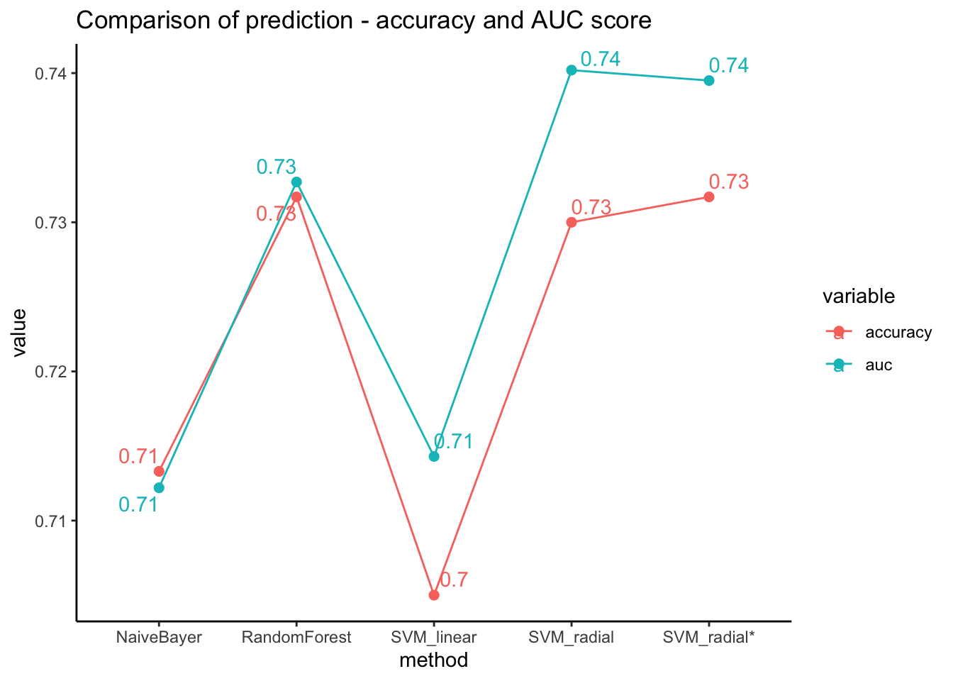
}

• We can demonstrate the model performances with a comparison plot. It shows that the performances are similar in both accuracy and auc score.

Code

data.frame(method = c("SVM_linear","SVM_radial","RandomForest","NaiveBayer"),
           accuracy = c(check_perf( factor(svm_linear_pred),"super")[[1]],
                        check_perf( factor(svm_radial_pred),"super")[[1]],
                        check_perf( factor(rf_pred),"super")[[1]],
                        check_perf( factor(nb_pred),"super")[[1]]),
           auc = c(check_perf( factor(svm_linear_pred),"super")[[2]],
                   check_perf( factor(svm_radial_pred),"super")[[2]],
                   check_perf( factor(rf_pred),"super")[[2]],
                   check_perf( factor(nb_pred),"super")[[2]])
           ) %>%  melt(id=c("method")) %>% 
  ggplot(aes(x=method, y=value, color=variable)) +
  geom_line(aes(group=variable)) + geom_point(size=2) + theme_classic() +
  geom_text_repel(aes(label=round(value,2)), position="dodge") +
  labs(title="Comparison of prediction - accuracy and AUC score")

6.7.3 Hyper-parameter tuning

• So far, we have used the default setting of the models. Using grid search approach, it is possible to find better parameters to boost the model performance.

  • In our case, support vector machine with radial kernel model achieved highest accuracy as well as auc score. We can test to find out whether changing parameters might improve its performance.

Code

# grid search for support vector machine
svm_tune <- tune(svm, 
                 Diabetes ~ Age+Sex+HighChol+BMI+ Smoker+HeartDiseaseorAttack + PhysActivity + Stroke + HighBP, 
                 data=train, 
                 kernel='radial', 
                 ranges = list(cost=c(0.01,0.1,1,1.5,2),
                               gamma=c(0.01,0.1,0.5,1,1.5,2)))

# set a new model with the best cost and gamma values
svm_radial_model_tune<- e1071::svm(Diabetes ~ Age+Sex+HighChol+BMI+ Smoker+HeartDiseaseorAttack + PhysActivity + Stroke + HighBP,
                        data = train, 
                        kernel='radial',
                        cost = summary(svm_tune)$best.parameters$cost,
                        gamma = summary(svm_tune)$best.parameters$gamma)
svm_radial_tune_pred = predict(svm_radial_model_tune, newdata = test[-18])

# re-visualize with the new model
data.frame(method = c("SVM_linear","SVM_radial","SVM_radial*","RandomForest","NaiveBayer"),
           accuracy = c(check_perf( factor(svm_linear_pred),"super")[[1]],
                        check_perf( factor(svm_radial_pred),"super")[[1]],
                        check_perf( factor(svm_radial_tune_pred),"super")[[1]],
                        check_perf( factor(rf_pred),"super")[[1]],
                        check_perf( factor(nb_pred),"super")[[1]]),
           auc = c(check_perf( factor(svm_linear_pred),"super")[[2]],
                   check_perf( factor(svm_radial_pred),"super")[[2]],
                   check_perf( factor(svm_radial_tune_pred),"super")[[2]],
                   check_perf( factor(rf_pred),"super")[[2]],
                   check_perf( factor(nb_pred),"super")[[2]])
           ) %>%  melt(id=c("method")) %>% 
  ggplot(aes(x=method, y=value, color=variable)) +
  geom_line(aes(group=variable)) + geom_point(size=2) + theme_classic() +
  geom_text_repel(aes(label=round(value,2)), position="dodge") +
  labs(title="Comparison of prediction - accuracy and AUC score")