2 Chapter 2. Hierarchical Clustering

2.1 Introduction

One of the most commonly applied unsupervised learning techniques is agglomerative, or hierarchical clustering.
- In this approach, we rely heavily on a distance metric that relates any two observations (pairs) in the data.
- Here is the algorithm for hierarchical clustering, in a nutshell. It is a ‘greedy’ algorithm:
  - We ‘initialize’ by assigning each subject to its own, solitary cluster.
  - At each step/stage, we merge the two clusters that are closest to each other – and we need to be more precise about ‘closest’
- Closest is defined using two pieces of information.
  - All subjects are assigned a distance from every other subject, similar to a matrix of distances between cities on a road map.
  - For now, Euclidean distance between two points in space will anchor our understanding.
  - Just so that we are clear, here is a sample Euclidean distance matrix for points \((0,0)\), \((0,3)\), \((4,0)\):
- Quite similar to a correlation matrix: common diagonal and symmetric entries.
- A correlation matrix is a good covariate similarity matrix
  - 1 minus the correlation would represent dissimilarity, or distance, as we are using the term

Code

pts <- matrix(c(0,0,0,3,4,0),3,2,byrow=T)
dists <- as.matrix(dist(pts))
dimnames(dists) <- list(c("(0,0)","(0,3)","(4,0)"),c("(0,0)","(0,3)","(4,0)"))
pander::pander(dists)

	(0,0)	(0,3)	(4,0)
(0,0)	0	3	4
(0,3)	3	0	5
(4,0)	4	5	0

2.1.1 Exercise 1

Exercise link

The distances are used to define how close two clusters are.
- Remember that at each stage we merge the two nearest clusters.
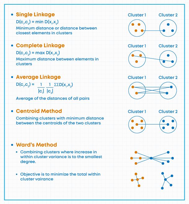
- Three most common ways to define nearest:
  - Minimum pair-wise distance
  - Maximum pair-wise distance
  - Minimum centroid distance
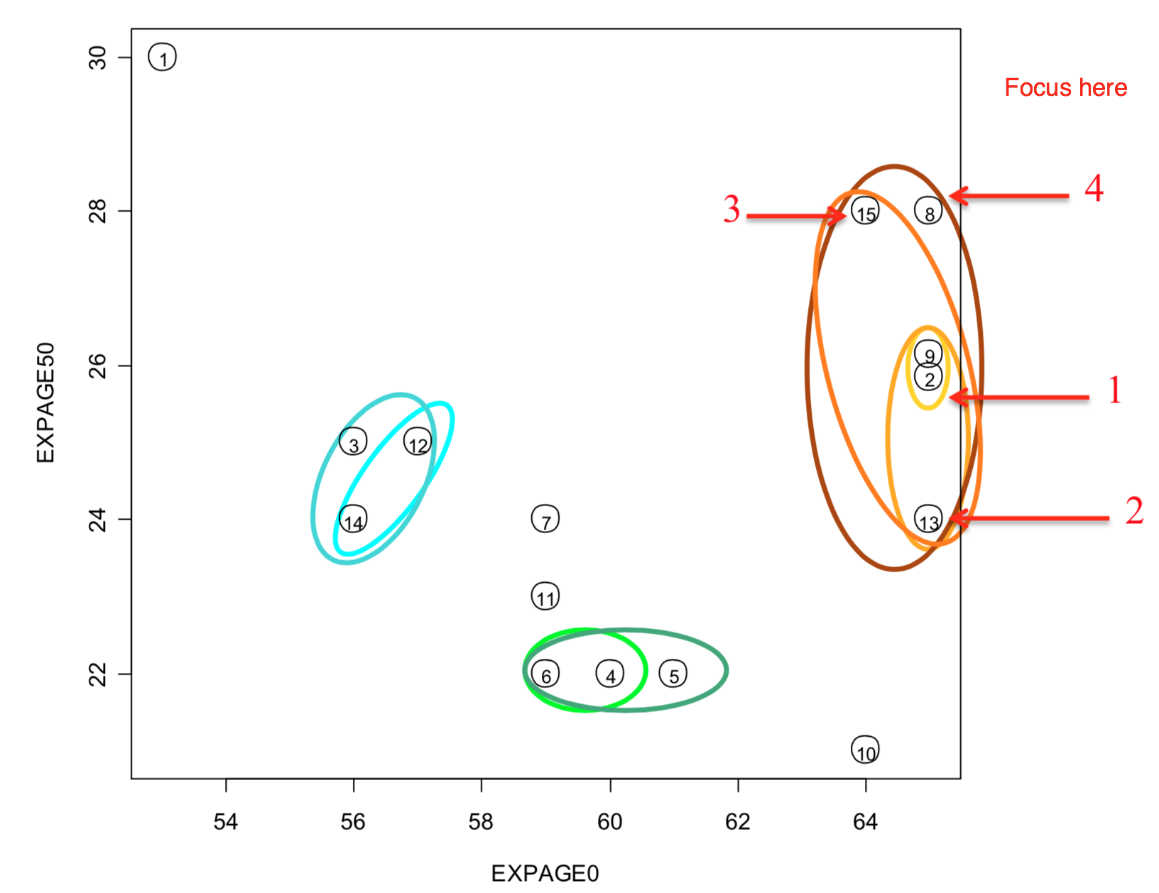
- Follow the agglomeration in yellow/orange/brown (ignoring other colors).
- Lightest loop represents the first agglomeration.
- The lines get progressively darker each join.
- Reminder: this original feature set was four-dimensional.
Minimum pair-wise distance
- For any two clusters, take one observation from each and determine their distance.
- Do this over and over, until you have identified the overall minimum pair-wise distance.
- This is the nearest neighbor method.
- In software, it is often called single linkage.
- Just to be clear, at each step of the algorithm, all possible pairs of clusters are evaluated to determine which two observations are closest.

NN Example with Male Life Expectancy data

Maximum pair-wise distance
- Nearest may be defined as the furthest (or maximum) distance between two clusters.
- All possible pairwise distances between elements (one from cluster A and one from B) are evaluated and the largest value is used as the distance between clusters A & B.
- This is sometimes called complete linkage and is also called furthest neighbor
  - NOTE: Think of this approach as insuring that two clusters that are joined are such that all elements contained in them are near all elements in the other cluster.
- This approach tends to create tight clumps, rather than ‘stringy’ ones that are quite common in the single linkage approach.
Centroid clustering
- Assigns each newly joined cluster a set of coordinate values based on the (multivariate) mean value (centroid) for all of the subjects contained within it.
- The centroid is recomputed after any merge.
- The distances are recomputed after any merge.
- NOTE: current hclust implementation of centroid method does not follow this algorithm exactly due to lack of original metric.

Image source

2.1.2 Example

5-cluster solution (we stop agglomerating when there are 5 clusters) for three different linkage methods
- Numbers are case ID
- Color is assigned cluster.
- Notice the ‘tightness’ of the clusters (or lack of it).

Code

maleLifeExp <- read.dta("./Datasets/malelifeexp.dta")  
hcl.single <- hclust(dist(maleLifeExp[,2:5]),meth='single')
hcl.complete <- hclust(dist(maleLifeExp[,2:5]),meth='complete')
hcl.centroid <- hclust(dist(maleLifeExp[,2:5]),meth='centroid')
hcl.ward <- hclust(dist(maleLifeExp[,2:5]),meth='ward.D2')  #for later

Code

factoextra::fviz_cluster(list(data=maleLifeExp[,2:5],cluster=cutree(hcl.single,5)),choose.vars=c(1,3),main="Single Linkage")

## Registered S3 methods overwritten by 'broom':
##   method            from  
##   tidy.glht         jtools
##   tidy.summary.glht jtools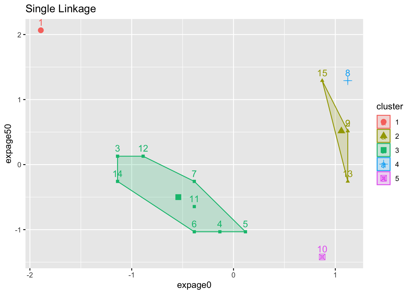

Code

factoextra::fviz_cluster(list(data=maleLifeExp[,2:5],cluster=cutree(hcl.complete,5)),choose.vars=c(1,3),main="Complete Linkage")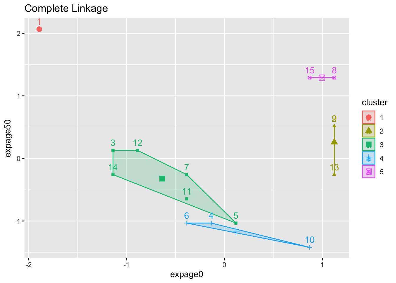

Code

factoextra::fviz_cluster(list(data=maleLifeExp[,2:5],cluster=cutree(hcl.centroid,5)),choose.vars=c(1,3),main="Centroid Linkage")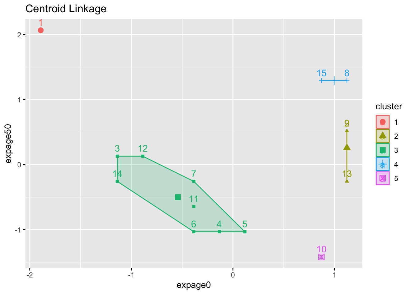

2.1.3 Exercise 2 and 3

Exercise link

Notes:
- Do we see an ‘error’ in the single linkage solution?
- Why is ID 15 (and not 8) part of the larger cluster below it?
- A look at the (Euclidean) distance matrix for IDs 8, 9, 15 reveals:
  - ID 9 is the closest element of the bottom cluster before the merge.
  - ID 15 is seen to be much closer to it (3.61 away), while ID 8 is further at 5.39.
- In the plot, you are only seeing the distance based on 2 of the 4 measures, so it is misleading.
  - ID 8 is closer to ID 9 on the plot.
  - ID 8 differs most from 9 for EXPAGE75.

Code

  dmat <- as.matrix(dist(maleLifeExp[c(8,9,15),2:5]))
  dimnames(dmat) <- list(c(8,9,15),c(8,9,15))
  pander::pander(dmat,digits=3)

	8	9	15
8	0	5.39	3.74
9	5.39	0	3.61
15	3.74	3.61	0

Confirm the above intuition by looking at the clustering in PCA space:

Code

factoextra::fviz_cluster(list(data=maleLifeExp[,2:5],cluster=cutree(hcl.single,5)),main="Single Linkage")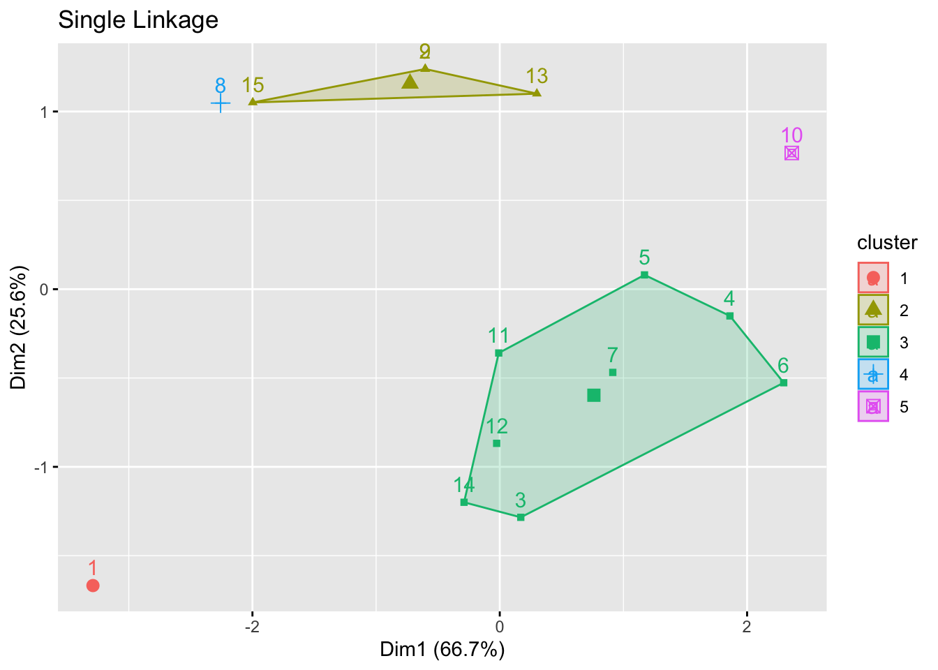

2.2 Ward’s method

In Ward’s method, the goal at any stage is to find two clusters to join such that a total sum of squares associated with the proposed groupings increases by the smallest amount possible (again, at every step).
At each stage of the clustering, you have assigned a ‘current set’ of group labels (call it a best guess).
Using those groups, if you ran an ANOVA, there would be a within groups error (squared and summed—across all features).
- Mathematically, assuming there are \(g\) groups, that squared, component-wise error is: \(E=\sum\limits_{m=1}^{g}{{{E}_{m}}}\), where \({{E}_{m}}=\sum\limits_{l=1}^{{{n}_{m}}}{\sum\limits_{k=1}^{p}{({{X}_{m,lk}}-{{{\bar{X}}}_{m,k}}}{{)}^{2}}}\) and \(n_m\) is the number of observations in the \(m^{th}\) group, \(p\) is the number of features, \(X_{m,lk}\) is the \(k^{th}\) feature of the \(l^{th}\) observation in the \(m^{th}\) group, and \({{\bar{X}}_{m,k}}\)is the mean of the \(k^{th}\) feature in group \(m\).
- For each \(m\), \(E_m\) is the sum of squared Euclidean distances of each element from its group mean.
Initially every observation is in its own cluster.
At each step in Ward’s method, we combine two of the groups, decreasing their total number from \(m\) to \(m-1\).
- We must look through every possible pair of clusters that could be combined, and re-compute \(E\) based on each new, potential clustering.
- Notation: \(E^0\) is the result of computing formula \(E\), above for the most recent configuration of clusters; \(E^{ij}\) is formula \(E\) evaluated with clusters \(i\) and \(j\) newly joined.
- Then we seek \(i\), \(j\), such that \(E^{ij}-E^0\) is minimized at every step. (a greedy algorithm)
Ward’s method is known to tend to form equal-sized clusters
- It is also known to be sensitive to outliers.

2.3 Agglomeration schedule, dendrogram

An agglomeration ‘schedule’ notes the point at which single elements and larger clusters are merged.
- This agglomeration over time produces a tree-like summary known as a dendrogram.
In the dendrogram, the distance for which a chosen agglomeration occurs is the natural scale on which to make comparisons
- Available for single, complete and centroid linkage

2.3.1 Example: single linkage, Male Life Expectancy

Code

plot(hcl.single,labels=maleLifeExp[,1])
mtext("distance @ pt. of merge",side=2,at=4.7,col=2,cex=.75, adj=.25, las=1)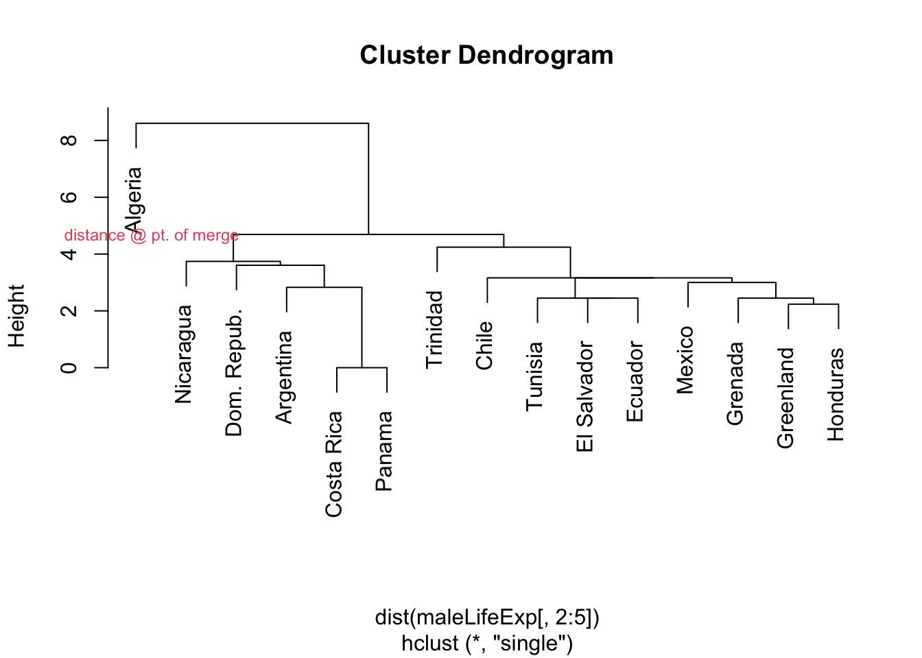

2.3.2 Exercise 4, and 5

Exercise link

Notes:
- For the bottom-most tree, Costa Rica & Panama are joined first (they seem to be identical – zero distance apart)
- This is followed by Argentina ‘much later’ (meaning at greater distance apart)
- …then Dom. Republic, then Nicaragua.
- Given the heights, Tunisia, El Salvador, and many others to the right were merged before Argentina joined the Costa Rica/Panama cluster.
- Algeria is a bit of a multivariate outlier.
  - It was the rightmost blue line at EXPAGE50 on the parallel coordinate plot on Handout 1, as it crossed from minimum to maximum level from AGEEXP0 to AGEEXP50.
  - Here, we see it is joined last, in part because it is so different from the other nations with respect to these measures.

2.3.3 Example: complete linkage, Male Life Expectancy

Code

plot(hcl.complete,labels=maleLifeExp[,1])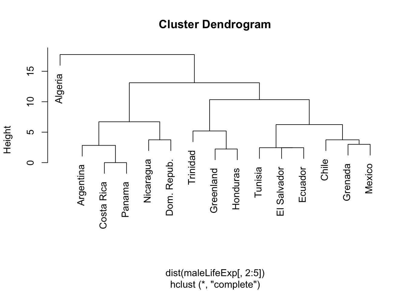

2.3.4 Exercise 6

Exercise link

Only small differences (from single linkage)

2.3.5 Example: Ward’s linkage, Male Life Expectancy

Code

plot(hcl.ward,labels=maleLifeExp[,1])
abline(h=12.5,col=2)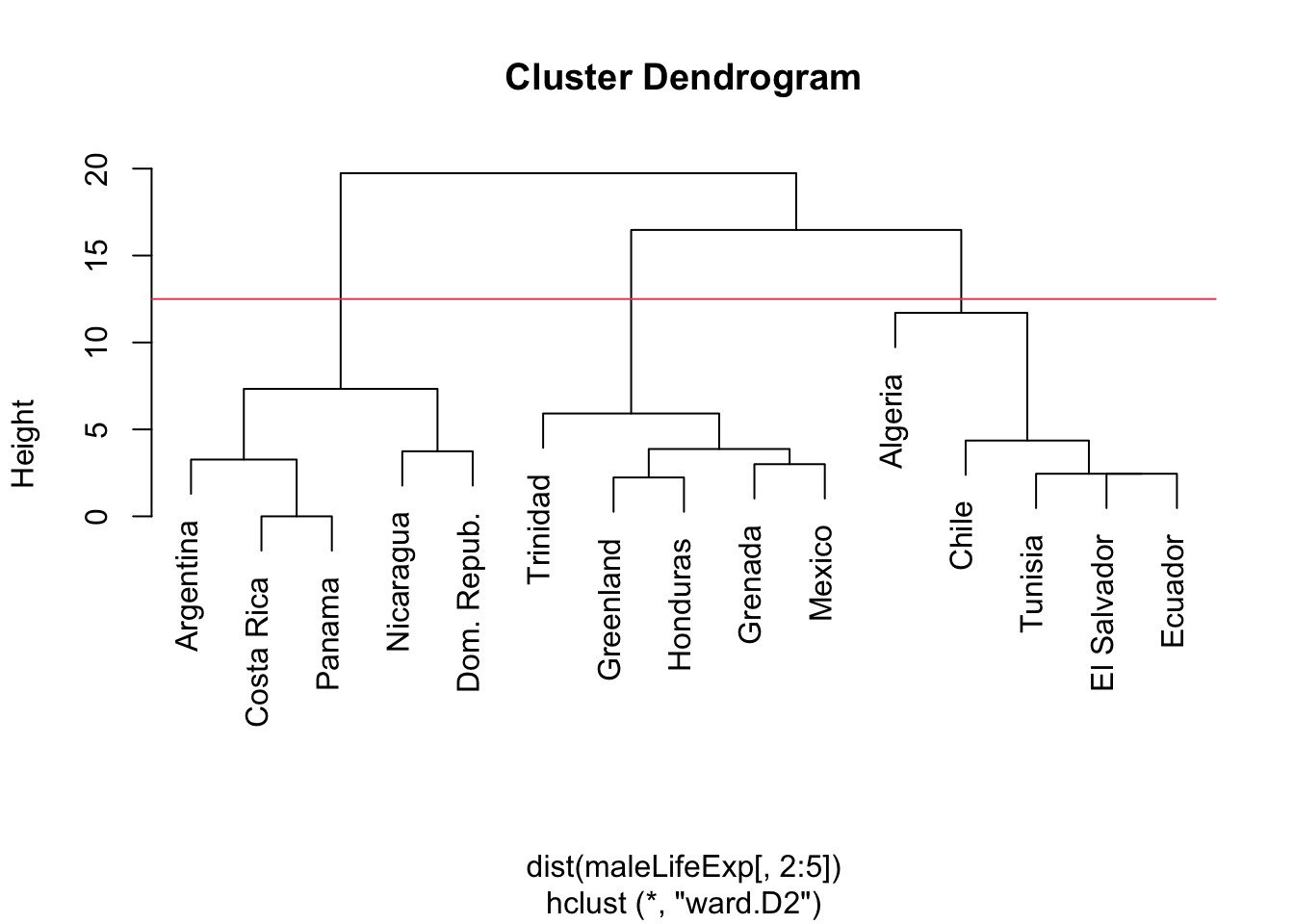

Notes:
- The minimized cost \(E^0-E^{ij}\) for each merge is the height of the dendrogram at that merge
- In the above agglomeration schedule, Algeria joins the rightmost cluster before the others have been joined, and this could change everything.
  - If we were to stop aggregating when there were three clusters, Algeria would be in a cluster with four nations.
  - Contrast this to the single or complete linkage solutions in which Algeria is in its own cluster until the final merge.

2.3.6 Choosing ‘cut points’ for the clustering

Once the hierarchical clustering is complete (all elements are joined), then we can examine the agglomeration tree to see whether there is a natural cut point at which we see that two very distinct branches are finally being merged.
- Think of taxonomy and the differentiation of species:
  - Humans are primates, mammals, and then vertebrates, and then animals, in the hierarchy.
  - At each stage of that hierarchy, very different creatures are being grouped together. E.g., mollusks are animals, too.
The biggest problem with hierarchical clustering is that it is not based strongly on a statistical model.
- Where do we set a break point (cut point) to form a reasonable number of clusters?
- And what do we say of the clusters that are created?
- Why do we think that these groupings are meaningful?
One way to address some of the above concerns is to apply substantive knowledge to the resulting clusters.
- If we look at the names of the nations clustered by life expectancy, we might have an idea of regional or development status effects.
- In general, we would hope to be able to assign meaningful names to the resulting clusters.
- But there are different perspectives on this:
  - If we cannot ‘name’ clusters then clustering may not be appropriate.
  - How will we justify any interpretation of the findings?

2.4 Importance of naming the clusters?

Groups may correspond to different levels of an outcome of interest, but it may be hard to use the typology if it cannot be described in terms of available measures reasonably easily.
- Can you answer the question, ‘what do these objects all have in common?’
- Alternatively, a clustering may be very useful for a ‘downstream’ process.
  - Consider market segmentation, in which the goal is to have a quick way to place a new customer in with similar customers, for ad targeting, e.g.
- Can you think of other applications in which naming the cluster is less important than finding the clusters?
- As in most of applied statistics, what you intend to do based on or with the analysis is crucial

2.4.1 Cluster naming example

Below is the 3-cluster single linkage result based on life expectancy
- Can you assign names to these clusters – esp. the right-most cluster?

Code

mlx <- maleLifeExp[,2:5]
rownames(mlx) <- maleLifeExp$country
factoextra::fviz_cluster(list(data=mlx,cluster=cutree(hcl.single,3)),repel=T,main="Single Linkage")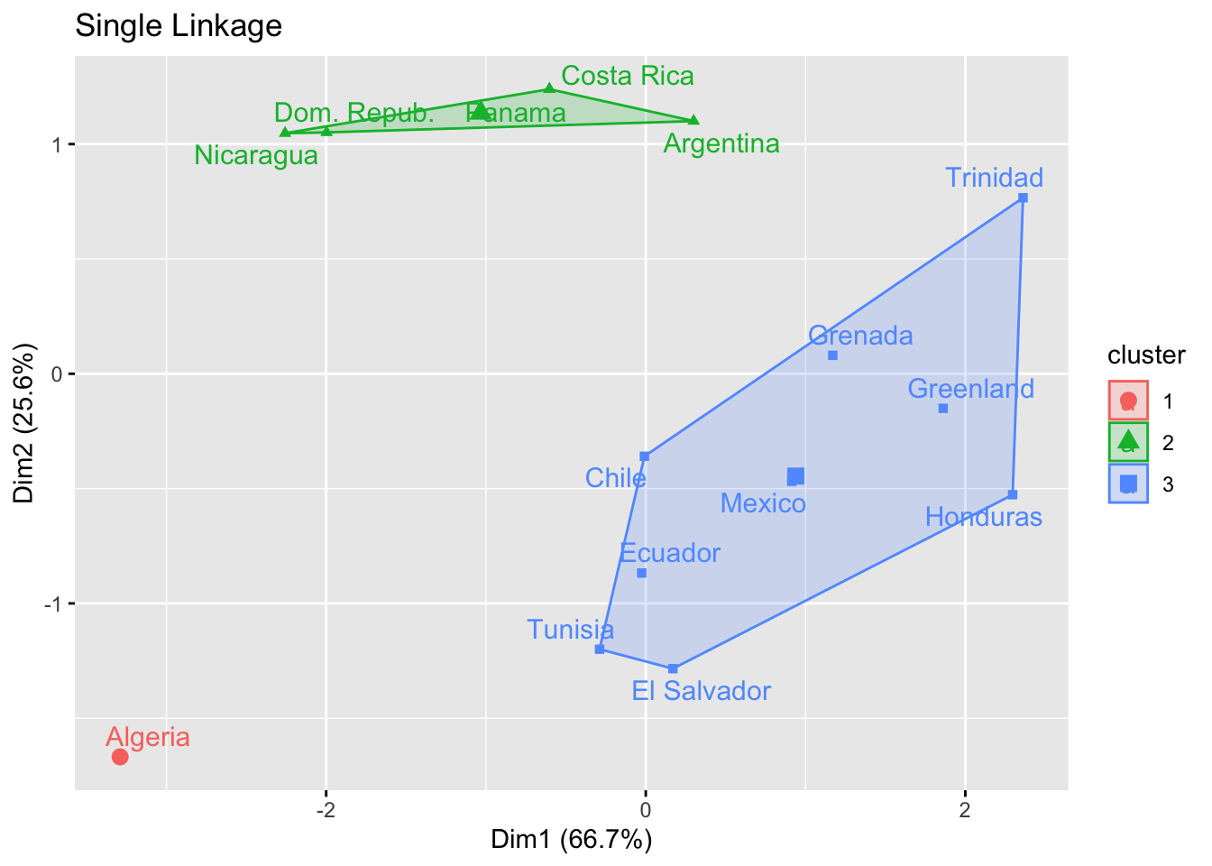

2.4.2 Comparing cluster solutions

We need a way to compare solutions
- Case in which we fix the number of clusters
  - Assign group labels for every observation
  - Cross-tabulate the group labels resulting from the different methods.
- The idea is to ‘cut’ (think: draw a horizontal line through) the dendrogram at a point that has the desired number of groups.
- Case in which it is tied to choosing the number of clusters is more complex

2.4.3 Comparison of three cluster solutions (life expectancy data)

Single vs. complete linkage

Code

lbls.single <- cutree(hcl.single,k=3)
lbls.complete <- cutree(hcl.complete,k=3)
lbls.ward <- cutree(hcl.ward,k=3)
xtabs(~lbls.single+lbls.complete)

##            lbls.complete
## lbls.single 1 2 3
##           1 1 0 0
##           2 0 5 0
##           3 0 0 9

2.4.4 Exercise 7

Exercise link

Suggests complete agreement on the cluster for the two approaches (all entries on the diagonal of the table)
Single vs. Ward’s method

Code

xtabs(~lbls.single+lbls.ward)

##            lbls.ward
## lbls.single 1 2 3
##           1 1 0 0
##           2 0 5 0
##           3 4 0 5

The entry ‘4’ in the (3,1) position suggests that Ward’s method assigned four nations to the same cluster as Algeria, while single linkage would have kept Algeria in it’s own separate cluster.

2.4.5 Corresponding dendrogram

Assignment differences should be readily apparent in the dendrogram (below, with the 3 cluster solution in red boxes):

Code

plot(hcl.ward,labels=maleLifeExp[,1])
rect.hclust(hcl.ward,k=3)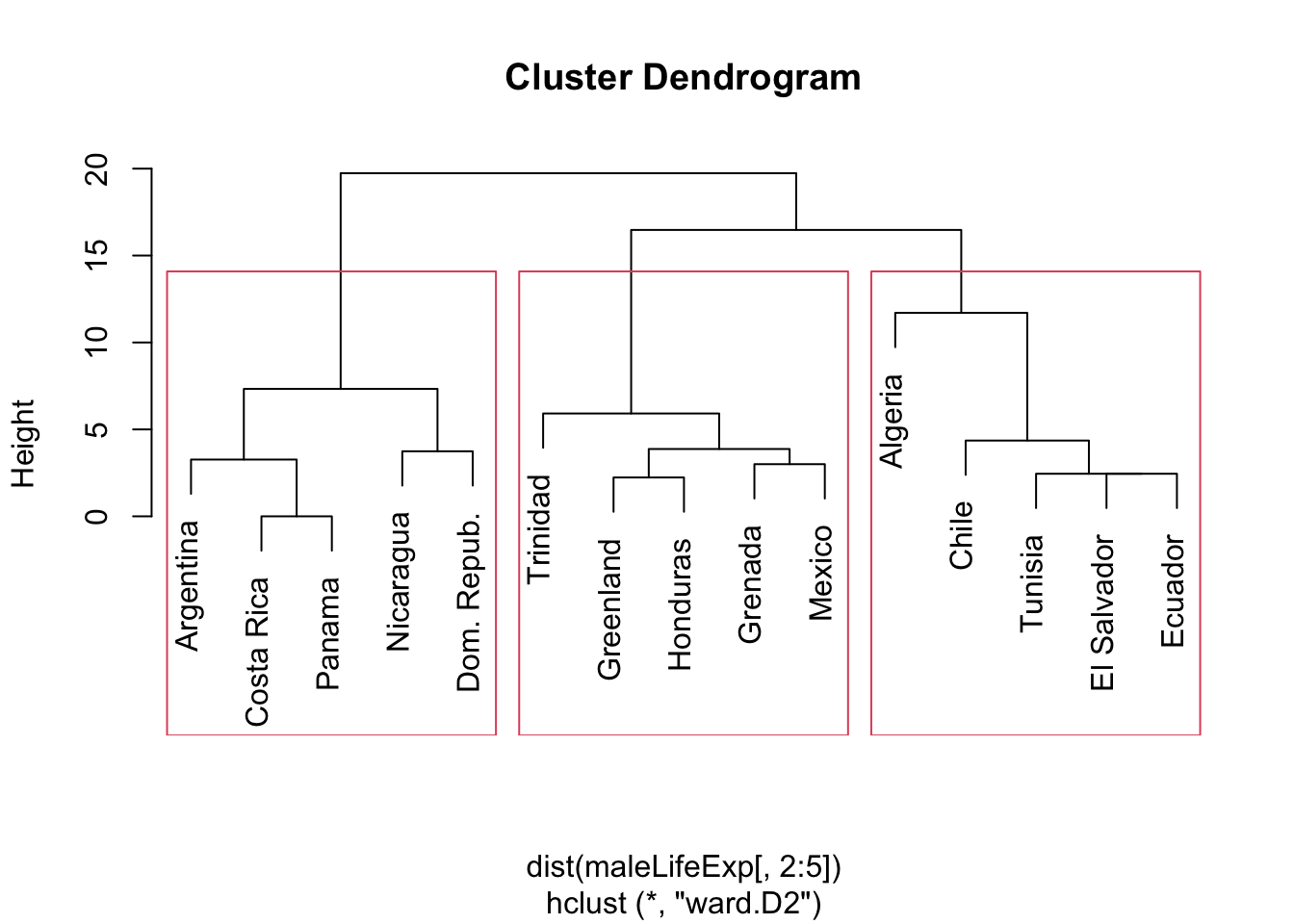

What if we had witnessed this crosstab:

Code

lbls.single.alt <- lbls.single
#swap
lbls.single.alt[lbls.single.alt==2] <- 4
lbls.single.alt[lbls.single.alt==3] <- 2
lbls.single.alt[lbls.single.alt==4] <- 3
xtabs(~lbls.single.alt+lbls.complete)

##                lbls.complete
## lbls.single.alt 1 2 3
##               1 1 0 0
##               2 0 0 9
##               3 0 5 0

This simply means that the labels have ‘switched’ but the cluster assignments are identical.
- There is still perfect agreement, even though it may not be immediately apparent if you just look at the diagonal.
- It can take a bit of work to sort this out, but it is possible to do so.

2.4.6 EXAMPLE: Eurowork (Industry %)

Code

eurowork <- read.dta("./Datasets/eurowork.dta")
eurowork$country <- substring(eurowork$country,1,10) #format issue
pander::pander(eurowork)

country	agr	min	man	ps	con	ser	fin	sps	tc
Austria	12.7	1.1	30.2	1.4	9	16.8	4.9	16.8	7
Belgium	3.3	0.9	27.6	0.9	8.2	19.1	6.2	26.6	7.2
Denmark	9.2	0.1	21.8	0.6	8.3	14.6	6.5	32.2	7.1
Finland	13	0.4	25.9	1.3	7.4	14.7	5.5	24.3	7.6
France	10.8	0.8	27.5	0.9	8.9	16.8	6	22.6	5.7
Ireland	23.2	1	20.7	1.3	7.5	16.8	2.8	20.8	6.1
Italy	15.9	0.6	27.6	0.5	10	18.1	1.6	20.1	5.7
Netherland	6.3	0.1	22.5	1	9.9	18	6.8	28.5	6.8
Norway	9	0.5	22.4	0.8	8.6	16.9	4.7	27.6	9.4
Sweden	6.1	0.4	25.9	0.8	7.2	14.4	6	32.4	6.8
Switzerlan	7.7	0.2	37.8	0.8	9.5	17.5	5.3	15.4	5.7
UK	2.7	1.4	30.2	1.4	6.9	16.9	5.7	28.3	6.4
W. Germany	6.7	1.3	35.8	0.9	7.3	14.4	5	22.3	6.1
Luxembourg	7.7	3.1	30.8	0.8	9.2	18.5	4.6	19.2	6.2
Greece	41.4	0.6	17.6	0.6	8.1	11.5	2.4	11	6.7
Portugal	27.8	0.3	24.5	0.6	8.4	13.3	2.7	16.7	5.7
Spain	22.9	0.8	28.5	0.7	11.5	9.7	8.5	11.8	5.5
Turkey	66.8	0.7	7.9	0.1	2.8	5.2	1.1	11.9	3.2
Bulgaria	23.6	1.9	32.3	0.6	7.9	8	0.7	18.2	6.7
Poland	31.1	2.5	25.7	0.9	8.4	7.5	0.9	16.1	6.9
Romania	34.7	2.1	30.1	0.6	8.7	5.9	1.3	11.7	5
Czechoslov	16.5	2.9	35.5	1.2	8.7	9.2	0.9	17.9	7
E. Germany	4.2	2.9	41.2	1.3	7.6	11.2	1.2	22.1	8.4
Hungary	21.7	3.1	29.6	1.9	8.2	9.4	0.9	17.2	8
USSR	23.7	1.4	25.8	0.6	9.2	6.1	0.5	23.6	9.3
Yugoslavia	48.7	1.5	16.8	1.1	4.9	6.4	11.3	5.3	4

Apply a squared Euclidean distance to standardized percentages.
- This keeps all industries on the same scale
- Use of z-scores has the effect of identifying an unusual mix of industries.
Here are the results from a centroid method clustering visualized in the dendrogram.
- NOTE: Stata cannot produce this dendrogram due to a ‘reversal’

Code

eurowork <- read.dta("./Datasets/eurowork.dta")
hcl.cent <- hclust(dist(scale(eurowork[,2:10]))^2,meth='centroid')
plot(hcl.cent,labels=eurowork[,1])
text(20,5,"Reversal",cex=.7,col=2,adj=0)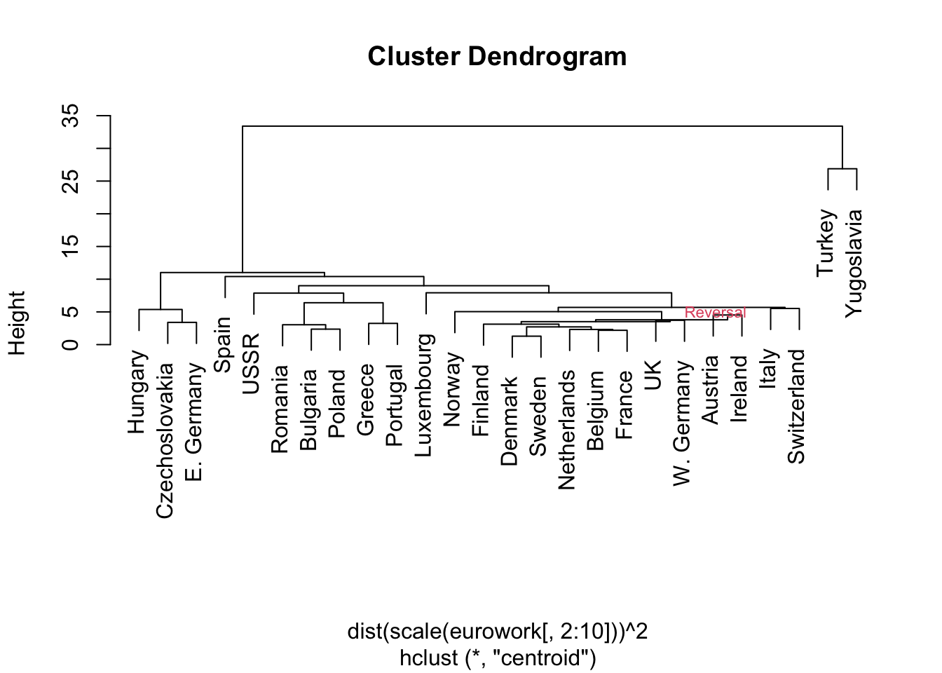

2.4.7 Exercise 7

Exercise link

There is an approximate East/West Europe divide
- Turkey and Yugoslavia the most disparate of the countries
  - Note: the data pre-date the fall of the Berlin Wall and the breakup of Yugoslavia
Below is a 9 cluster cut of the same data.
- This seemed to keep most intuitive clumps together.
- We might expect a different configuration for Western European countries (this was not born out in the clustering)
  - E.g., why are Greece and Portugal ‘close’?
- Uneven cluster sizes are common to hierarchical clustering
  - But centroid & complete linkages are supposed to limit this somewhat.

Code

lbls.cent <- as.matrix(cutree(hcl.cent,k=9))
rownames(lbls.cent) <- eurowork$country
colnames(lbls.cent)<-c("Cluster")
pander::pander(lbls.cent)

	Cluster
Austria	1
Belgium	1
Denmark	1
Finland	1
France	1
Ireland	1
Italy	1
Netherlands	1
Norway	1
Sweden	1
Switzerland	1
UK	1
W. Germany	1
Luxembourg	2
Greece	3
Portugal	3
Spain	4
Turkey	5
Bulgaria	6
Poland	6
Romania	6
Czechoslovakia	7
E. Germany	7
Hungary	7
USSR	8
Yugoslavia	9

Code

plot(hcl.cent,labels=eurowork[,1])
rect.hclust(hcl.cent,k=9)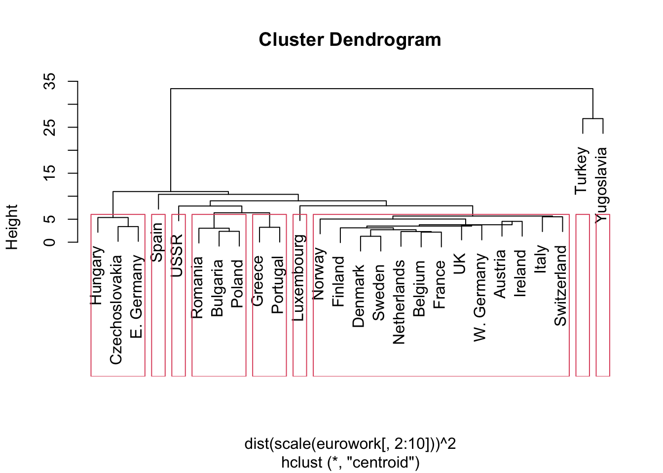

2.5 Dimensionality Reduction

Principal Components (PCs) let us look at the clusters in a space with reduced dimensionality.
- We will use the correlation matrix for eurowork (why?)
- We chose the number of factors based on the eigenvalues
  - A common criterion is to keep all factors with eigenvalue at least one, or use the scree plot to look for a break
- The eigenvalue criterion chose three factors, and we saved ‘scores’ for principal components for each country.
- Plot the data using these scores and compare the ‘natural’ clusters we think we see with the centroid-linkage-based clusters.
  - We found ‘natural’ groupings using the \(2^{nd}\) and \(3^{rd}\) principle component scores.

Code

pc.euro <- princomp(eurowork[,-1],cor=T)$scores
plot(pc.euro[,2:3],col=rainbow(9)[lbls.cent],xlim=c(-4,2),cex=.75)
text(pc.euro[,2:3],labels=eurowork[,1],col=rainbow(9)[lbls.cent],pos=2)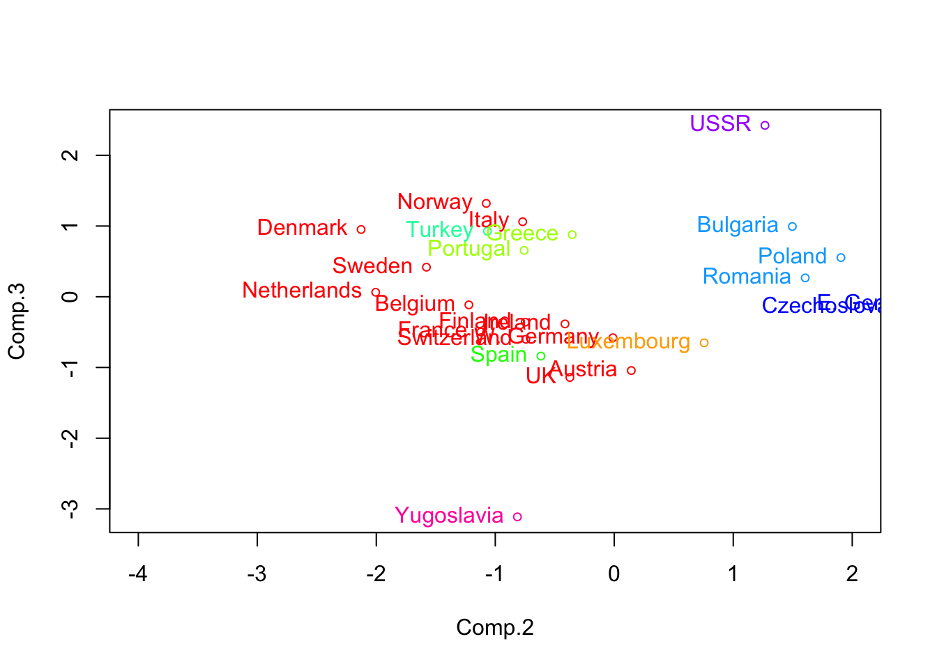

2.5.1 Exercise 8

Exercise link

2.5.2 Optimization approaches to clustering

A ‘good’ clustering is one in which clusters are well separated and fairly homogeneous within themselves. More formally:
- Homogeneity: objects within a group should have a cohesive structure.
  - Assume the groups have already been assigned.
  - We can quantify the homogeneity within each group using a sum of squares criterion (like we do in ANOVA, and this comes right out of Ward’s criterion).
  - Say there are \(p\) features. Compute \(W=\sum\limits_{m=1}^{g}\sum\limits_{l=1}^{n_m}(\mathbf{x}_{ml}-\bar{\mathbf{x}}_m)(\mathbf{x}_{ml}-\bar{\mathbf{x}}_m)'\), where \(n_m\) is the number of observations in the \(m^{th}\) group, \({{\mathbf{x}}_{ml}}\) is the \(p\times 1\) column vector representing the \(p\) features in the \(l^{th}\) observation in that group, and \(\bar{\mathbf{x}}_m\) is the mean feature vector for that group.
  - Reminder: a vector is just a shorthand for an ordered list of values or symbols.
- If there are p features, \(x_1,x_2,\ldots,x_p\), then we can stack them in a column, in that order, and call the stacked values by a ‘bolded’ ( vector) name:

\[\mathbf{x}=\left( \begin{matrix} {{x}_{1}} \\ {{x}_{2}} \\ \vdots \\ {{x}_{p}} \\ \end{matrix} \right) \]

We can represent row vectors as the ‘transposed’ version of the column vector: \(\mathbf{{x}'}=\left( {{x}_{1}},{{x}_{2}},\ldots ,{{x}_{p}} \right)\) - Lastly, we can multiply these vectors, element by element

\[ \mathbf{x{x}'}=\left( \begin{matrix} {{x}_{1}}{{x}_{1}} & {{x}_{1}}{{x}_{2}} & \cdots & {{x}_{1}}{{x}_{p}} \\ {{x}_{2}}{{x}_{1}} & {{x}_{2}}{{x}_{2}} & \cdots & {{x}_{2}}{{x}_{p}} \\ \vdots & \vdots & \ddots & \vdots \\ {{x}_{p}}{{x}_{1}} & {{x}_{p}}{{x}_{2}} & \cdots & {{x}_{p}}{{x}_{p}} \\ \end{matrix} \right) \]

Let’s ‘unpack’ the vector product in the equation for \(W\) a bit further.
- A \(p\times 1\) column vector is multiplying a \(1\times p\) row vector.
  - Note from that formula: \(l\) is observation number; \(m\) is group number.
- The \(k^{th}\) entry of the vector is the deviation of the kth feature from the group mean for that feature.
- The vector product generates a \(p\times p\) matrix, as above, analogous to a correlation matrix.
- The \((j,k)^{th}\) entry of the matrix corresponds to \(({{x}_{m,lj}}-{{\bar{x}}_{m,j}})({{x}_{m,lk}}-{{\bar{x}}_{m,k}})\)
  - Where \(x_{m,lj}\), \(x_{m,lk}\) are the \(j^{th}\) and \(k^{th}\) entries in the feature vector, and the other terms are group means for those features.
When \(j=k\), on the diagonal of the matrix, this is a squared deviation term that is part of a variance calculation; otherwise, it is a covariance term (in a larger computation).
- The matrix, \(W\), contains the sum of these ‘simpler’ matrices both within and across the groups.
- To the extent that each observation is reasonably close to its group mean, these entries will be small, and the overall matrix of entries will be very small as well.
- So homogeneity can be formalized as some function of this matrix \(W\).
Separation: the groups should be well isolated from each other. - This suggests that the variation between groups should be large.
- There is an analogous matrix that captures the components of between group variation. It is called the between-group dispersion matrix, and is given by \(B=\sum\limits_{m=1}^{g}{n_m}(\bar{\mathbf{x}}_m - \bar{\mathbf{x}})(\bar{\mathbf{x}}_m-\bar{\mathbf{x}})'\), where the p-vectors \(\bar{\mathbf{x}}_m\) and \(\bar{\mathbf{x}}\) represent the mean vector for group \(m\) and for the entire dataset, respectively.
The sum is weighted ‘up’ by \(n_m\), so that each observation contributes equally (larger groups count more).
- Both \(W\) and \(B\) are \(p\times p\) matrices, and they actually decompose the total dispersion matrix, \(T\), given below.
  - These matrix decompositions are crucial to the theory underlying MANOVA.
Let \(T=\sum\limits_{m=1}^{g}\sum\limits_{l=1}^{n_m}(\mathbf{x}_{ml}-\bar{\mathbf{x}})(\mathbf{x}_{ml}-\bar{\mathbf{x}})'\).
- Then \(T=W+B\). [Matrices ‘add’ element-wise]
- These terms \(W\) and \(B\) are important because they measure homogeneity and separation with respect to the total dispersion, \(T\).

2.5.3 Exercise 9

Exercise link

Functions of these components are used for:
- Partitioning observations into clusters (optimization criteria)
- Choosing the number of clusters
Optimization method I: minimize trace(W)
- The trace (‘tr’) of a matrix is simply the sum of its diagonal terms, which translates very nicely (capturing variance-like terms only) into:
  
  \[ tr(W)=\sum\limits_{m=1}^{g}{\sum\limits_{l=1}^{{{n}_{m}}}{\sum\limits_{k=1}^{p}{({{x}_{m,lk}}-{{{\bar{x}}}_{m,k}}}{{)}^{2}}}} \]
This is Ward’s clustering criterion.
- DO NOT think, however, that what we are about to do is the same as hierarchical clustering using Ward’s criterion.
- You will see how it differs.

2.5.4 PARTITIONING

In an optimization method, we want to choose the best of all possible ways to partition \(n\) observations into \(g\) groups.
- Each partition is an assignment of group labels, as the examples illustrate:

An optimization method, in theory:
- Enumerates each possible partition
- Evaluates some criterion that reflects homogeneity and/or separation
- Picks the partition (group label assignment) corresponding to the ‘best’ value of the criterion.

2.5.5 Partition example in simple setting

We observe 2 features on 6 objects: \[({{\mathbf{x}}_{1}},{{\mathbf{x}}_{2}},{{\mathbf{x}}_{3}},{{\mathbf{x}}_{4}},{{\mathbf{x}}_{5}},{{\mathbf{x}}_{6}})=\left( \begin{matrix} 1 & 0 & 0 & 1 & 2 & 2 \\ 0 & 1 & 0 & 2 & 1 & 2 \\ \end{matrix} \right)\].
Under partition 1, above, \[{{\bar{x}}_{1}}=\frac{1}{4}\left\{ \left( \begin{matrix} 1 \\ 0 \\ \end{matrix} \right)+\left( \begin{matrix} 0 \\ 0 \\ \end{matrix} \right)+\left( \begin{matrix} 1 \\ 2 \\ \end{matrix} \right)+\left( \begin{matrix} 2 \\ 2 \\ \end{matrix} \right) \right\}=\left( \begin{matrix} 1 \\ 1 \\ \end{matrix} \right)\] and \[{{\bar{x}}_{2}}=\frac{1}{2}\left\{ \left( \begin{matrix} 0 \\ 1 \\ \end{matrix} \right)+\left( \begin{matrix} 2 \\ 1 \\ \end{matrix} \right) \right\}=\left( \begin{matrix} 1 \\ 1 \\ \end{matrix} \right)\]
Yields deviations from the mean (note change in notation): \((\mathbf{x}_{11}-\bar{\mathbf{x}}_1,\mathbf{x}_{21}-\bar{\mathbf{x}}_2,\mathbf{x}_{12}-\bar{\mathbf{x}}_1,\mathbf{x}_{13}-\bar{\mathbf{x}}_1,\mathbf{x}_{22}-\bar{\mathbf{x}}_2,\mathbf{x}_{14}-\bar{\mathbf{x}}_1)\) \(=\left( \begin{matrix} 0 & -1 & -1 & 0 & 1 & 1 \\ -1 & 0 & -1 & 1 & 0 & 1 \\ \end{matrix} \right)\)
In terms of \(W=\sum\limits_{m=1}^{g}\sum\limits_{l=1}^{n_m}(\mathbf{x}_{ml}-\bar{\mathbf{x}}_m)(\mathbf{x}_{ml}-\bar{\mathbf{x}}_m)'\), we have: \[ W=\left( \begin{matrix} 0 \\ -1 \\ \end{matrix} \right)\left( \begin{matrix} 0 & -1 \\ \end{matrix} \right)+\left( \begin{matrix} -1 \\ 0 \\ \end{matrix} \right)\left( \begin{matrix} -1 & 0 \\ \end{matrix} \right)+\left( \begin{matrix} -1 \\ -1 \\ \end{matrix} \right) \left( \begin{matrix} -1 & -1 \\ \end{matrix} \right) \] \[ +\left( \begin{matrix} 0 \\ 1 \\ \end{matrix} \right)\left( \begin{matrix} 0 & 1 \\ \end{matrix} \right)+\left( \begin{matrix} 1 \\ 0 \\ \end{matrix} \right)\left( \begin{matrix} 1 & 0 \\ \end{matrix} \right)+\left( \begin{matrix} 1 \\ 1 \\ \end{matrix} \right)\left( \begin{matrix} 1 & 1 \\ \end{matrix} \right) \]

\[ W=\left( \begin{matrix} 0\cdot 0 & 0\cdot (-1) \\ -1\cdot 0 & -1\cdot (-1) \\ \end{matrix} \right)+\left( \begin{matrix} -1\cdot (-1) & -1\cdot 0 \\ 0\cdot (-1) & 0\cdot 0 \\ \end{matrix} \right) \]

\[ +\left( \begin{matrix} -1\cdot (-1) & -1\cdot (-1) \\ -1\cdot (-1) & -1\cdot (-1) \\ \end{matrix} \right) +\left( \begin{matrix} 0\cdot 0 & 0\cdot 1 \\ 1\cdot 0 & 1\cdot 1 \\ \end{matrix} \right) \]

\[ +\left( \begin{matrix} 1\cdot 1 & 1\cdot 0 \\ 0\cdot 1 & 0\cdot 0 \\ \end{matrix} \right)+\left( \begin{matrix} 1\cdot 1 & 1\cdot 1 \\ 1\cdot 1 & 1\cdot 1 \\ \end{matrix} \right) \]

[note: centered dot is ‘multiply’]

\[ W=\left( \begin{matrix} 0 & 0 \\ 0 & 1 \\ \end{matrix} \right)+\left( \begin{matrix} 1 & 0 \\ 0 & 0 \\ \end{matrix} \right)+\left( \begin{matrix} 1 & 1 \\ 1 & 1 \\ \end{matrix} \right)+\left( \begin{matrix} 0 & 0 \\ 0 & 1 \\ \end{matrix} \right)+\left( \begin{matrix} 1 & 0 \\ 0 & 0 \\ \end{matrix} \right)+\left( \begin{matrix} 1 & 1 \\ 1 & 1 \\ \end{matrix} \right) \]

\[ =\left( \begin{matrix} 4 & 2 \\ 2 & 4 \\ \end{matrix} \right) \]

So tr(W) = 4+4=8.
Under partition 2, above, omitting details

\[ W=\left( \begin{matrix} .44 & -.22 \\ -.22 & .11 \\ \end{matrix} \right)+\left( \begin{matrix} .11 & -.22 \\ -.22 & .44 \\ \end{matrix} \right)+\left( \begin{matrix} .11 & .11 \\ .11 & .11 \\ \end{matrix} \right) \]

\[ +\left( \begin{matrix} .44 & -.22 \\ -.22 & .11 \\ \end{matrix} \right)+\left( \begin{matrix} .11 & -.22 \\ -.22 & .44 \\ \end{matrix} \right)+\left( \begin{matrix} .11 & .11 \\ .11 & .11 \\ \end{matrix} \right) \]

\[ =\left( \begin{matrix} 1.33 & -.67 \\ -.67 & 1.33 \\ \end{matrix} \right) \]

so \(tr(W)=1.33+1.33=2.67\)

2.5.6 Notes

\(tr(W)\) is SMALLER under partition 2, so this partition would be preferred.
- To fully explore all possible partitions, we would have to look at 15 possible group assignments, then look at tr(W) and choose the partition that minimized this criterion.
- For most problems of any decent size, however, there is a combinatorial explosion:
  - For n=15 and g=3, there are over 2 million partitions, which is computationally feasible on a modern PC.
  - For n=100 and g=5, there are \(10^{68}\) partitions, so we will not be able to evaluate them all.

2.5.7 Alternative: Recursive Partitioning

The algorithm starts by assigning all observations to one of \(g\) clusters.
1. This could be done at random, or via an initial set of proposed group means
2. Group means are calculated
3. Elements are reassigned such that they are in the cluster that is closest to them (under the latest partition)
4. Go back to step 2. Repeat until no more reassignments occur.

2.5.8 K-means

Recursive partitioning executed in this manner has been called k-means, and has the following properties:
- Under certain conditions, it is consistent: if there are \(g\) groups in the data, and a very simple (normal) error process, this algorithm will ‘converge’ on (or find) the proper group means.
- Under certain conditions, is equivalent to minimizing \(tr(W)\).
- It is somewhat sensitive to initial conditions, so in practice, researchers often run it several times with different starting values (initial group means).
Other properties of \(tr(W)\) minimization methods (such as k-means):
- Minimizes the sum of the squared Euclidean distances between observations and their group mean.
- Not scale-invariant (will give a different solution if some items in the feature set are rescaled).
- The method tends to find spherical clusters.

2.5.9 Exercise 10

Exercise link

2.5.10 Examples (R setup)

Common to look at a range of methods and number of clusters
- Here, we are trying to understand a process using all available data (not withholding - yet)

Code

set.seed(2011001)
km.penguins.3<-kmeans(penguins[,3:5],3)
km.penguins.4<-kmeans(penguins[,3:5],4)
set.seed(2011)
km.crabs.4<-kmeans(crabs[,-(1:3)],4)
km.crabs.7<-kmeans(crabs[,-(1:3)],7)
km.euro.4<-kmeans(eurowork[,-1],4)
km.euro.7<-kmeans(eurowork[,-1],7)
km.life.2<-kmeans(maleLifeExp[,2:5],2)
km.life.3<-kmeans(maleLifeExp[,2:5],3)

penguins: look at g=3,4:

Code

par(mfrow=c(1,2))
plot(penguins[,c("bill_length_mm","flipper_length_mm")],col=km.penguins.3$clust,pch=1,cex=1.5,lwd=2)
plot(penguins[,c("bill_length_mm","flipper_length_mm")],col=km.penguins.4$clust,pch=1,cex=1.5,lwd=2)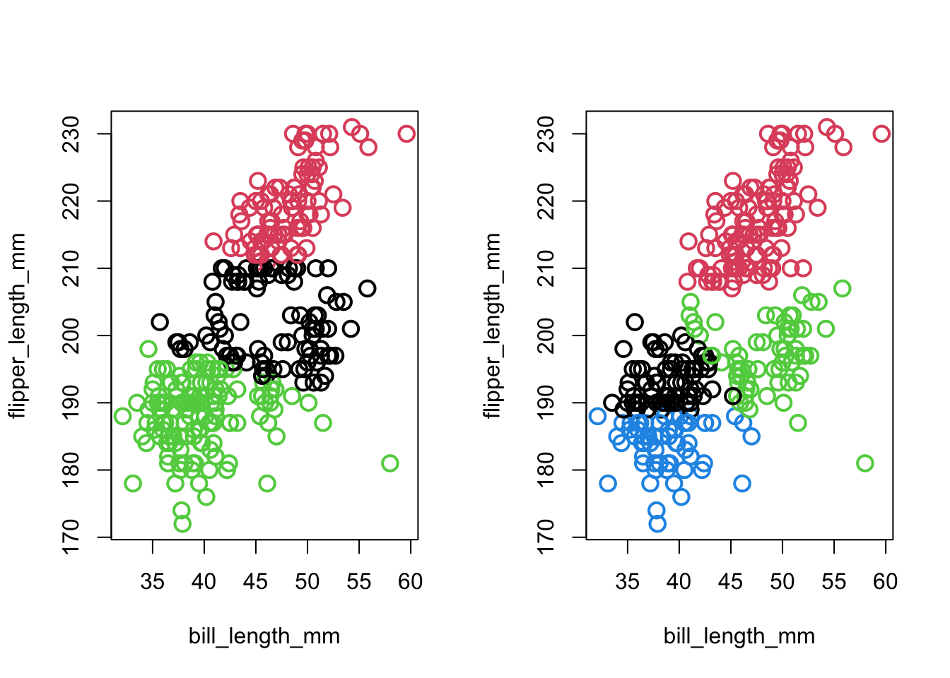

Crabs: look at g=4,7:

Code

par(mfrow=c(1,2))
plot(crabs[,5:6],col=km.crabs.4$clust,pch=1,cex=1.5,lwd=2)
plot(crabs[,5:6],col=km.crabs.7$clust,pch=1,cex=1.5,lwd=2)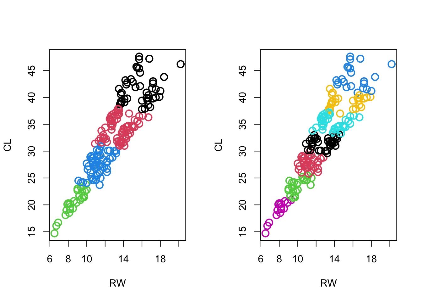

MaleLifeExp: g=2,3:

Code

par(mfrow=c(1,2))
plot(maleLifeExp[,c(2,4)],col=km.life.2$clust,pch=1,cex=1.5,lwd=2)
plot(maleLifeExp[,c(2,4)],col=km.life.3$clust,pch=1,cex=1.5,lwd=2)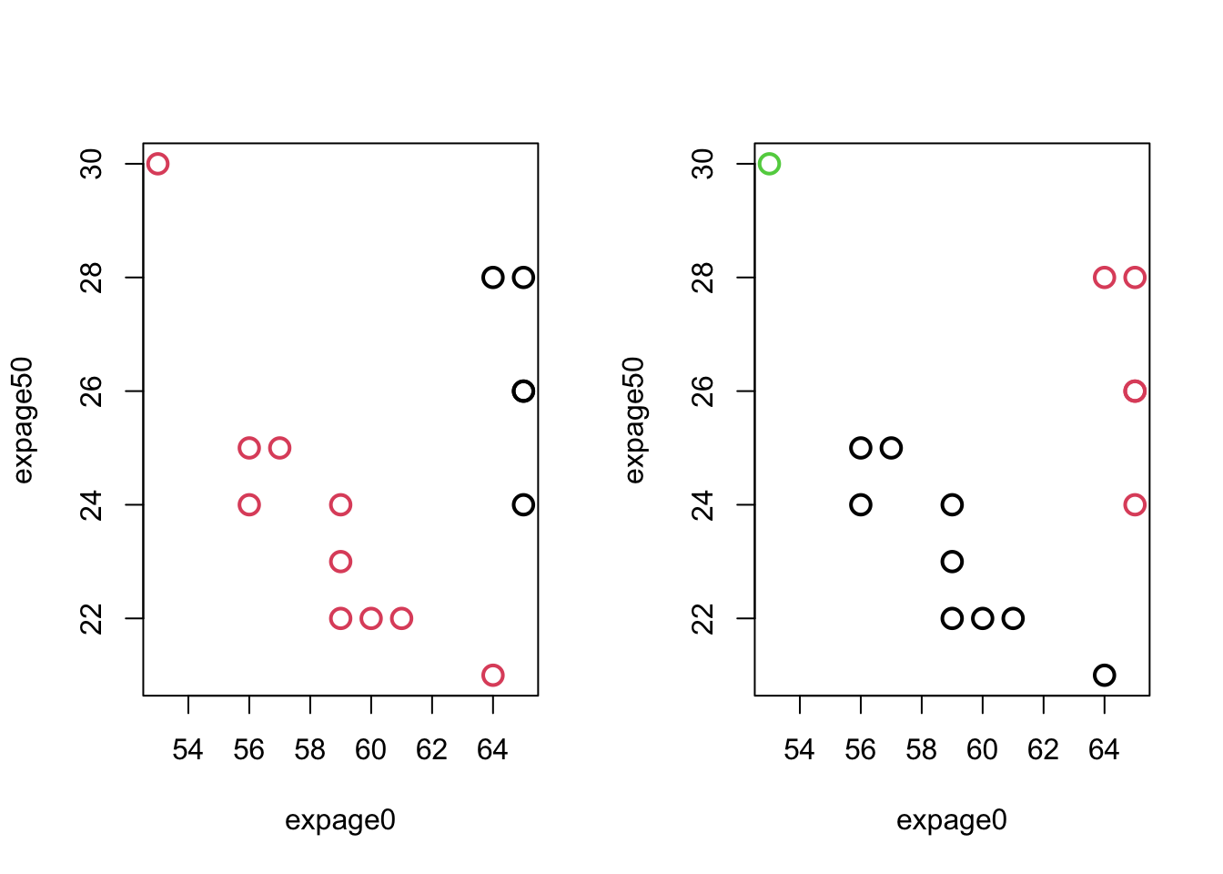

Eurowork (PCs): g=4,7:

Code

par(mfrow=c(1,2))
pc.euro <- princomp(eurowork[,-1])$scores
plot(pc.euro[,2:3],col=km.euro.4$clust,pch='.',type='n')
text(pc.euro[,2:3],as.character(eurowork[,1]),col=km.euro.4$clust,cex=.8)
plot(pc.euro[,2:3],col=km.euro.7$clust,pch='.',type='n')
text(pc.euro[,2:3],as.character(eurowork[,1]),col=km.euro.7$clust,cex=.8)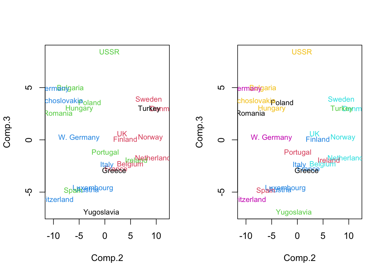

Code

par(mfrow=c(1,1))

2.6 Optimization method II: minimize det(W)

\(det(W)\) is a more complex combination of the terms in the matrix W reflecting the covariation as well as the variances.
- We often describe this approach as maximizing \(det(T)/det(W)\), but T is the same for all possible partitions of n individuals into g groups, so this is equivalent.
\(det(T)/det(W)\) is the reciprocal of Wilk’s Lambda (from MANOVA): large values of this measure indicate differences in multivariate groups.
This approach can identify elliptical clusters and is scale-invariant.
It tends to produce clusters that have an equal number of objects and are the same shape.
Hard to find a software implementation
- R’s mclust package implements a hierarchical approach that evaluates det(W) at each agglomeration stage (method ‘EEE’)

2.7 Choosing the number of clusters

The choice of the number of clusters in the population is a hard problem, but can be guided by the total amount of separation relative to the total amount of variation.
- These are roughly equivalent to \(R^2\) calculations, but with more than one feature, these relationships are based on summaries of matrix entries, such as tr(W).
- The concepts of homogeneity and separation were used to develop the following adequacy index, \(C(g)\) (Calinki&Harabasz criterion):

\[ C(g)=\frac{{\scriptstyle{}^{tr(B)}\!\!\diagup\!\!{}_{g-1}\;}}{{\scriptstyle{}^{tr(W)}\!\!\diagup\!\!{}_{n-g}\;}} \]

If we were in one dimension - a single feature only - then this is the mean square between (msb) groups divided by the mean square within (msw), or the F-ratio of explained to unexplained variability from ANOVA/regression.
In multiple dimensions, this is the sum of the msb to the sum of the msw estimates based on a full set of univariate ANOVAs.
- I will sometimes write this as C(g)=(\(\Sigma\) msb)/(\(\Sigma\)msw).
- In software, one has to identify the msb and msw components often given in an ‘ANOVA’ portion of k-means clustering output.
- The goal is to find g such that C(g) is maximized.
NbClust package in R evaluates about 20 different indices.
- Useful on practice to evaluate many different criteria in choosing number of clusters
- Option to pick the number that is optimal for majority of given criteria is available.
- Examples that follow may yield slightly different k-means solutions due to starting seeds and iterative (internal) algortihm.

2.7.1 Examples: C(g) on (k-means fits)

penguins data:

Code

NbC.penguins <- NbClust(data=penguins[,3:5], distance = "euclidean", min.nc=2, max.nc=10,method = "kmeans",index="ch")
plot(2:10,NbC.penguins$All.index,type='l',xlab='Number of Clusters',ylab='C(g)')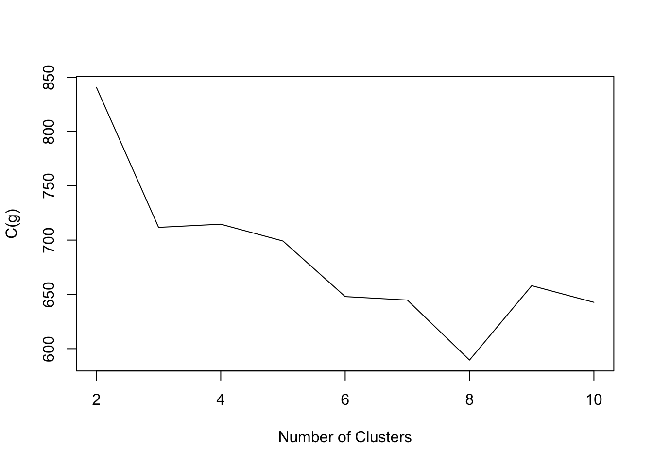

2.7.2 Exercise 11

Exercise link

Crabs data:

Code

NbC.crabs<- NbClust(data=crabs[,-(1:3)], distance = "euclidean", min.nc=2, max.nc=10,method = "kmeans",index="ch")
plot(2:10,NbC.crabs$All.index,type='l',xlab='Number of Clusters',ylab='C(g)')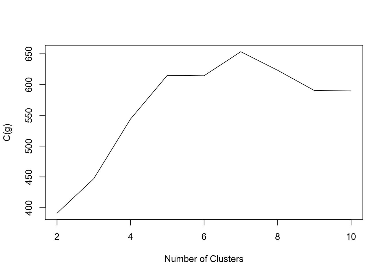

MaleLifeExp data:

Code

NbC.life<- NbClust(data=maleLifeExp[,2:5], distance = "euclidean", min.nc=2, max.nc=10,method = "kmeans",index="ch")
plot(2:10,NbC.life$All.index,type='l',xlab='Number of Clusters',ylab='C(g)')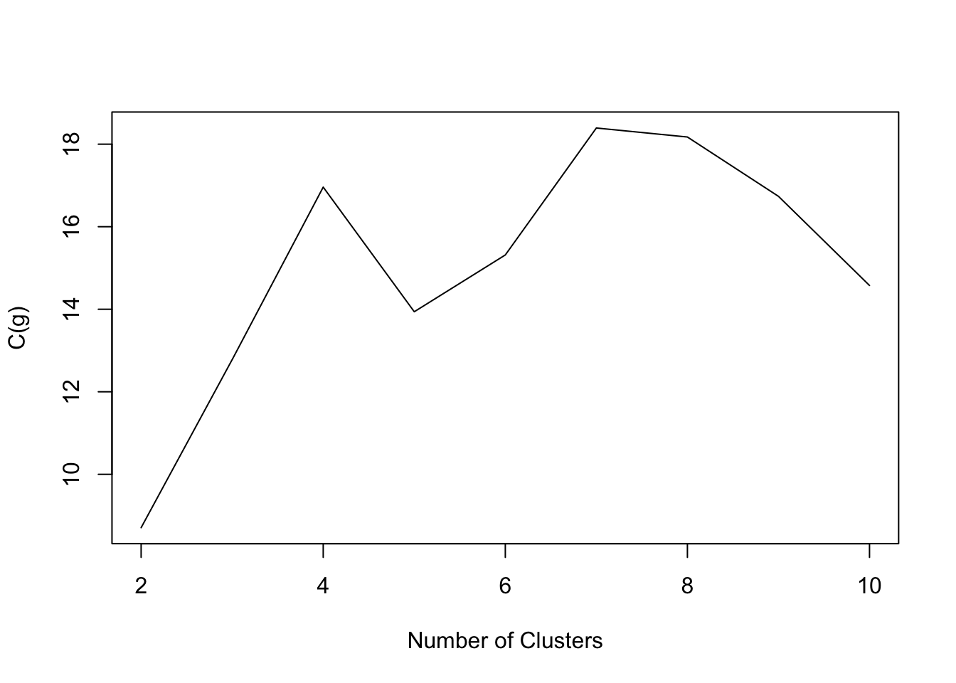

Eurowork data:

Code

NbC.euro<- NbClust(data=eurowork[,-1], distance = "euclidean", min.nc=2, max.nc=10,method = "kmeans",index="ch")
plot(2:10,NbC.euro$All.index,type='l',xlab='Number of Clusters',ylab='C(g)')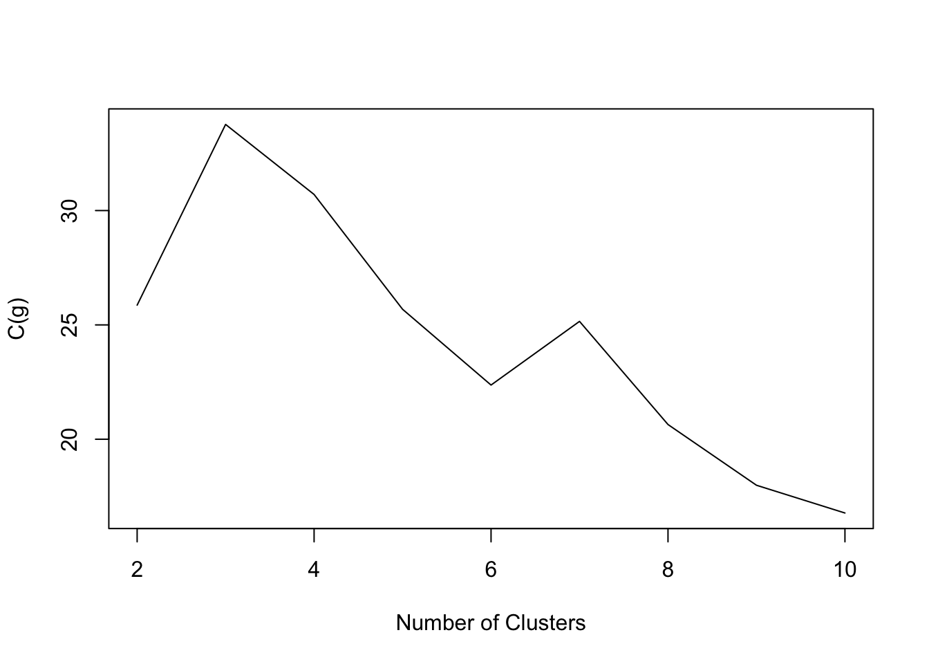

2.7.3 Rand index

RECALL the ‘label switching’ that occurs with clustering. Changing the cluster labels around is a lot of work.
The Rand index was developed to quantify the amount of agreement between two clustering solutions without appealing to a relabeling directly.
The Rand index is the proportion of pairs of observations that agree with respect to the clustering.
If \(i\) and \(j\) are two observations, and \(C_1\) and \(C_2\) are two different clustering solutions, then their labels can be written lab(\(C_1\),i), lab(\(C_2\),i), lab(\(C_1\),j), lab(\(C_2\),j): these are the labels for observation i in clustering \(C_1\) and \(C_2\) followed by the labels for observation j in clustering \(C_1\) and \(C_2\).
- The clustering solutions agree positively when lab(\(C_1\),i)=lab(\(C_1\),j) AND lab(\(C_2\),i)=lab(\(C_2\),j). They are in the same cluster, regardless of the clustering solution.
- The clustering solutions agree negatively when lab(\(C_1\),i) \(\neq\) lab(\(C_1\),j) AND lab(\(C_2\),i) \(\neq\) lab(\(C_2\),j). They are in different clusters, regardless of the clustering solution.
The Rand index can then be defined as:

\[ I_R=\frac{\left[ \begin{aligned} & \sum\limits_{i,j:i\ne j}{I\{lab({{C}_{1}},i)=lab({{C}_{1}},j)}\wedge lab({{C}_{2}},i)=lab({{C}_{2}},j)\}+ \\ & \sum\limits_{i,j:i\ne j}{I\{lab({{C}_{1}},i)\ne lab({{C}_{1}},j)}\wedge lab({{C}_{2}},i)\ne lab({{C}_{2}},j)\} \end{aligned} \right]}{\left( \begin{matrix} n \\ 2 \\ \end{matrix} \right)} \]

where

\[\left( \begin{matrix} n \\ 2 \\ \end{matrix} \right)\] is the number of pairs of observations we can draw from the full dataset and ‘^’ means ‘and.’

2.7.4 Exercise 12

Exercise link

2.7.5 DISCUSSION/EXAMPLE

Implementation of Rand Index requires care (typo in Brian Evett’s Cluster Analysis book, e.g., p. 182.)
Comparing hierarchical clustering with complete linkage to k-means, both with a 4 cluster solution, yields:

Code

comp.penguins.4 <- cutree(hclust(dist(penguins[,3:5]),meth='complete'),4)
xtabs(~comp.penguins.4+km.penguins.4$clust)

##                km.penguins.4$clust
## comp.penguins.4  1  2  3  4
##               1  1  0 35 28
##               2 77  0 11 37
##               3  0 79 20  0
##               4  0 45  0  0

Code

phyclust::RRand(comp.penguins.4,km.penguins.4$clust)

##    Rand adjRand  Eindex 
##  0.7703  0.4247  0.1513

One can compute the Rand index comparing potential clustering solutions with ‘known’ or ‘correct’ labeling.
- E.g., a three cluster solution using k-means for the penguins data – compared to the known species:

Code

phyclust::RRand(km.penguins.3$clust,as.numeric(penguins$species))

##    Rand adjRand  Eindex 
##  0.7843  0.5275  0.2476

Notes:
- Agreement of two clusterings does not imply you are closer to the ‘truth’ – just clustering in the same way.
- More sophisticated versions of the Rand Index exist
  - Adjusted Rand index corrects the above proportion for expectations under chance agreement.

2.8 Lab

Lab link

2.9 Appendix

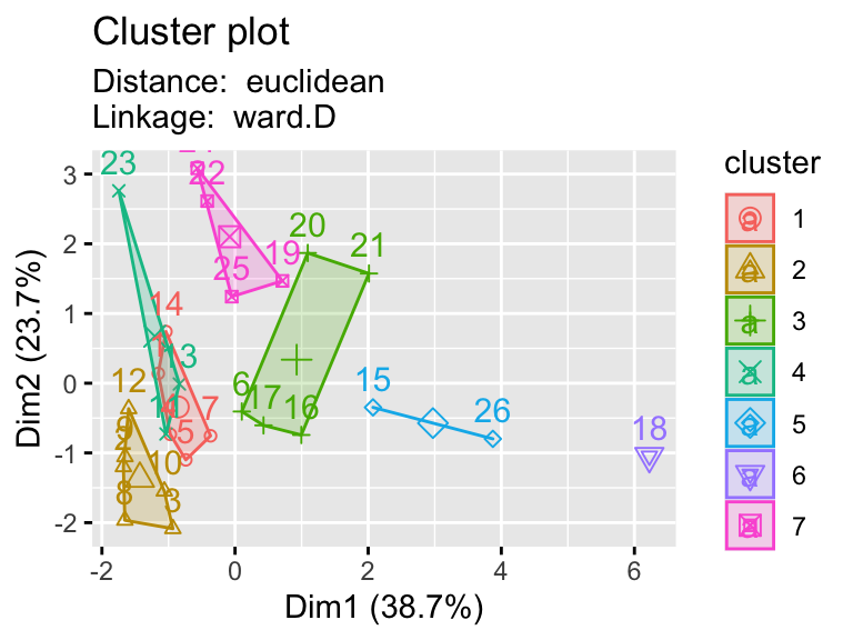
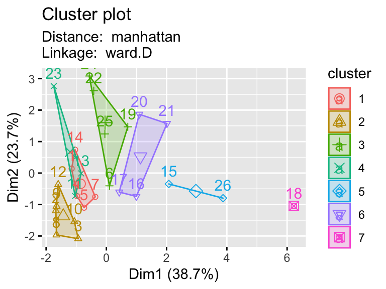
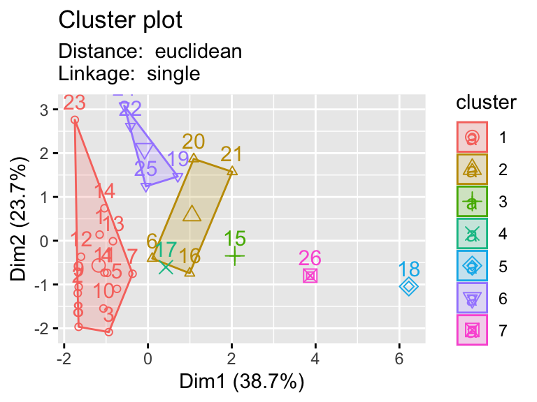
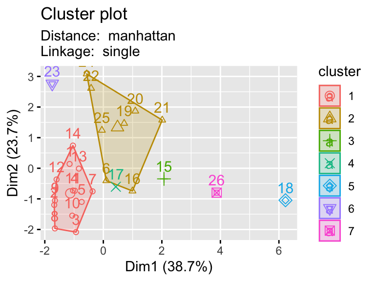
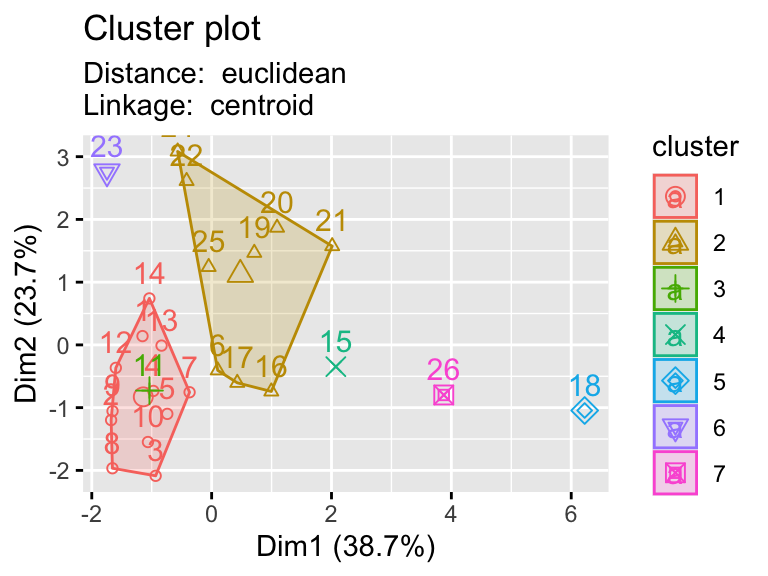
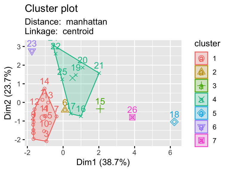
2.9.1 Testing multiple pairs of methods

Using a function to visualize different clustering methods can be useful as we have lots of parameters that we can explore.

Code

# import data
library(cluster)
eurowork <- read.dta("./Datasets/eurowork.dta")

# plotting k-means clustering
kmean_plot <- function(data, cluster){
  kmeans.re <- kmeans(data, centers = cluster)
  fviz_cluster(list(data = data, cluster = kmeans.re$cluster))
}

# plotting hierarchical clustering
hier_plot <- function(data, distance, linkage, cluster){
  d <- dist(eurowork[,-1], method = distance)
  hc5 <- hclust(d, method = linkage )
  sub_grp <- cutree(hc5, k = cluster)
  fviz_cluster(list(data = data, cluster = sub_grp),
               subtitle= paste("Distance: ", distance, "\nLinkage: ", linkage))
}

# testing plots
#kmean_plot(eurowork[,-1], 3) 
#hier_plot(eurowork[,-1],"euclidean","ward.D2", 3)

# plotting hierarchical clustering with different linkages
linkages <- c("ward.D","single","centroid")
distances <- c("euclidean","manhattan")
for (linkage in linkages){
  for(distance in distances){
    print(hier_plot(eurowork[,-1], distance, linkage, 7))
  }
}