Chapter 5 Hypothesis Testing
5.1 Common Hypothesis Testing for Six Sigma
Although not comprehensive, this chapter discusses the most common hypothesis testing techniques a Six Sigma professional normally handles. It also assumes that you have the basic knowledge behind Hypothesis Testing such as Null and Alternative hypothesis, alpha and beta risks, Type I and II errors, confidence level, and so on. With that out of the way, let’s get right into the tests.
5.2 1-Sample t Test
Let’s create a vector with some random data using the rnorm function, like this:
set.seed(1)
x <- rnorm(30,67.8,2.5)
Checking for x:
x## [1] 66.23387 68.25911 65.71093 71.78820 68.62377 65.74883
## [7] 69.01857 69.64581 69.23945 67.03653 71.57945 68.77461
## [13] 66.24690 62.26325 70.61233 67.68767 67.75952 70.15959
## [19] 69.85305 69.28475 70.09744 69.75534 67.98641 62.82662
## [25] 69.34956 67.65968 67.41051 64.12312 66.60462 68.84485Let’s then look into the summary statistics of this vector:
summary(x)## Min. 1st Qu. Median Mean 3rd Qu. Max.
## 62.26 66.71 68.44 68.01 69.57 71.79To run a non-directional 1-sample t test, we can execute the following code. Let’s assume that this vector contains the heights (in inches) of a given demographic. Let’s test if the \(\mu\) (true population mean) is equal to 68.5.
t.test(x, mu=68.5, conf.level = 0.95)##
## One Sample t-test
##
## data: x
## t = -1.1708, df = 29, p-value = 0.2512
## alternative hypothesis: true mean is not equal to 68.5
## 95 percent confidence interval:
## 67.14346 68.86883
## sample estimates:
## mean of x
## 68.00615The 1-sample t test above shows the results. For this data set, our p-value is greater than the set 0.05 (5%) alpha risk, therefore we fail to reject the Null Hypothesis, stating that there is not enough evidence to conclude that the true mean differs from 68.5 at the 5% level of significance.
5.3 2-Sample t Test
Let’s create another vector y, also using the rnorm function in R.
set.seed(1)
y <- rnorm(30,63.4,2)
A quick check of the data in y:
y## [1] 62.14709 63.76729 61.72874 66.59056 64.05902 61.75906
## [7] 64.37486 64.87665 64.55156 62.78922 66.42356 64.17969
## [13] 62.15752 58.97060 65.64986 63.31013 63.36762 65.28767
## [19] 65.04244 64.58780 65.23795 64.96427 63.54913 59.42130
## [25] 64.63965 63.28774 63.08841 60.45850 62.44370 64.23588Now let’s run a non-directional 2-sample t test between x and y, testing for the Alternative Hypothesis that the means between x and y are different.
t.test(x, y, mu=0, conf.level = 0.95)##
## Welch Two Sample t-test
##
## data: x and y
## t = 8.2219, df = 55.334, p-value = 3.637e-11
## alternative hypothesis: true difference in means is not equal to 0
## 95 percent confidence interval:
## 3.358852 5.523606
## sample estimates:
## mean of x mean of y
## 68.00615 63.56492The p-value in this case is extremely low. Therefore, we reject the Null Hypothesis in favour of the Alternative. We can conclude that the means differ at the 0.05 (5%) level of significance.
TIP: Notice that the Alternative Hypothesis states that the “true difference in means is not equal to 0.” This is the same as saying that they are different. If the true means were equal, their difference would have been zero.
5.4 One-Way ANOVA
First things first, we need to load a few packages for some great visuals on this test. Here they are:
library(reshape2)
library(gplots)
library(ggpubr)
library(ggthemes)
library(Rmisc)
The One-Way ANOVA looks into the differences among two or more population means in a statistical test involving a single factor. For this example, let’s create three vectors, like this:
T180 <- c(12.8,12.4,13.2,11.9)
T200 <- c(13.4,13.9,13.6,14.0)
T220 <- c(16.3,14.6,15.1,16.2)
These are three sets of responses in viscosity given temperatures in F. Let’s have a look at these vectors as a data frame. We can create a data frame by running the following code:
df <- data.frame(T180,T200,T220)Let’s see what this data frame looks like:
df## T180 T200 T220
## 1 12.8 13.4 16.3
## 2 12.4 13.9 14.6
## 3 13.2 13.6 15.1
## 4 11.9 14.0 16.2Now let’s “melt” this data frame and give the variables and values a name. We will use the melt function to achieve this. The x axis is for temperatures while the y axis is for viscosity.
data <- melt(df, id.vars = NULL,
             variable.name = "Temperature",
             value.name = "Viscosity")
We can then run a comparative boxplots chart to see how these three data sets look compared to each other in terms of central tendency and spread.
ggboxplot(title = "Boxplots of Temperatures and Viscosity",
          data, x = "Temperature", y = "Viscosity",
          color = "Temperature",
          palette = c("blue", "orange", "red"),
          order = c("T180", "T200", "T220"),
          ylab = "Viscosity", xlab = "Temperature")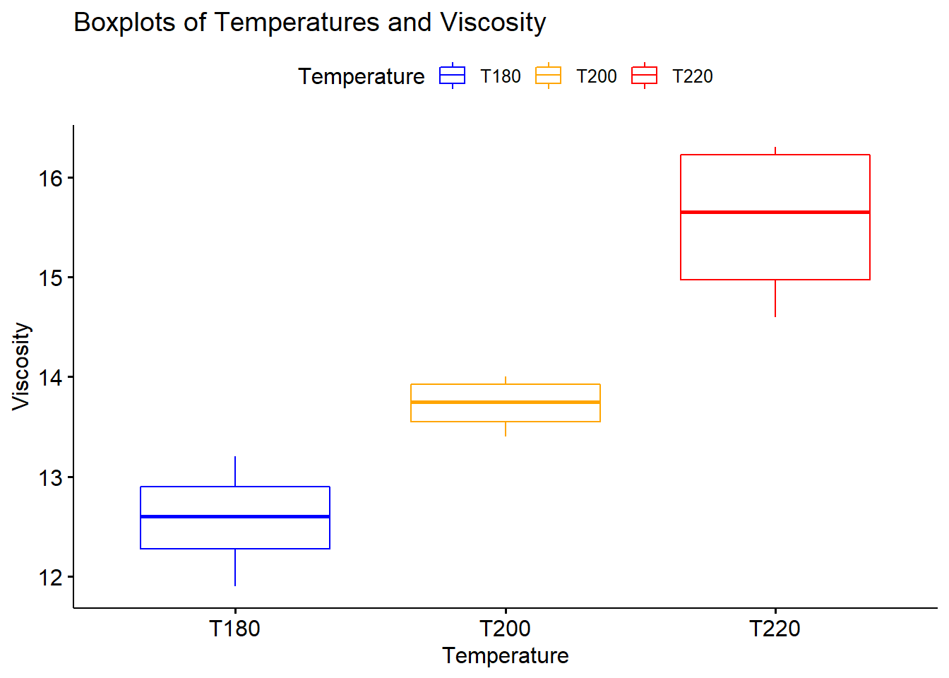
We can also run a plot that showcases the three data sets’ means and their confidence intervals. Pay attention and check if the confidence intervals overlap (one or more variables). If they don’t, we have an indication that the means differ. We’ll confirm this with the actual One-Way ANOVA test.
TIP: We should always consider the size of the differences to validate if they have practical implications.
ggline(title = "Plot of Means and Confidence Interval",
       data, x = "Temperature", y = "Viscosity",
       add = c("mean_se", "jitter"),
       order = c("T180", "T200", "T220"),
       ylab = "Viscosity", xlab = "Temperature")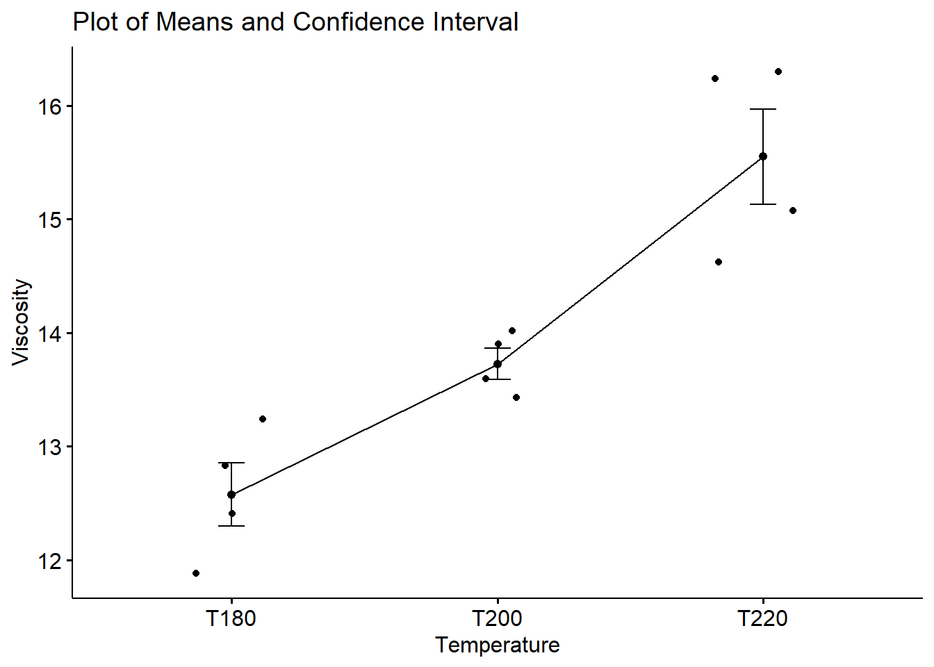
Finally, let’s run the One-Way ANOVA test and confirm, by looking at our p-value, if one or more of these data sets’ means differences are statistically significant from at least one another; in other words, let’s check if one or more temperature setting has an impact on the response variable viscosity.
res.aov <- aov(Viscosity~Temperature, data = data)
summary(res.aov)
## Df Sum Sq Mean Sq F value Pr(>F)
## Temperature 2 18.005 9.002 24.97 0.000212 ***
## Residuals 9 3.245 0.361
## ---
## Signif. codes:
## 0 '***' 0.001 '**' 0.01 '*' 0.05 '.' 0.1 ' ' 1Notice that the p-value (Pr(>F)) of 0.000212 is lower than the alpha risk of 0.05. In this example, we reject the Null Hypothesis and conclude that temperature affects the response variable viscosity.
5.5 1 Proportion Test
Let’s assume that the marketing department of a large organization is trying to test if their latest campaign on Facebook has yielded the expected results. They have targeted 500 people of a specific demographic, and 61 of those targeted have responded favourably to the campaign by purchasing the offered product. This marketing department claims that this is a better outcome than the previous year’s campaign that yielded a 10.8% favourability index.
Let’s break the information down first; this is what the example offers:
- number of trials: 500
- number of successes: 61
- targeted proportion: 10.8%
We can use the prop.test to perform the 1 proportion test, like this:
res <- prop.test(x = 61, n = 500, p = 0.108,
                 alternative = "greater",
                 conf.level = 0.95)
Running the object res will show the test results:
res##
## 1-sample proportions test with continuity correction
##
## data: 61 out of 500, null probability 0.108
## X-squared = 0.87714, df = 1, p-value = 0.1745
## alternative hypothesis: true p is greater than 0.108
## 95 percent confidence interval:
## 0.09902766 1.00000000
## sample estimates:
## p
## 0.122Given that our test is about the expected favourability index being greater than 10.8%, notice that we’ve used the argument alternative = “greater”.
The p-value for this test is 0.1745, therefore greater than the set alpha risk of 0.05 (for a confidence level of 95%). In this case, we fail to reject the Null Hypothesis. There is no statistical significance to support the marketing department’s claim that this year’s campaign has been better than last year’s.
5.6 2 Proportions Test
Let’s now consider the 2 proportions test. In this example, we’ll be looking at two different groups of people in the same city. The first group was interviewed in an affluent neighbourhood, the second, in an impoverished neighbourhood. The survey asked both groups if they thought that level of education yields better outcomes in life. The research team was testing if the affluent neighborhood group would answer “YES” proportionally more than the second group.
Here’s the break down of the information:
241 out of 600 interviewed (first group, affluent neighbourhood) said “YES” to the question.
160 out of 500 interviewed (second group, impoverished neighbourhood) said “YES” to the question.
The Null Hypothesis is that there is no difference between the proportions of “YES”es answered by both groups. The Alternative Hypothesis is that the first group will answer with more “YES”es to this specific question, proportionally speaking.
Here’s the code for the test:
res <- prop.test(x = c(241, 160), n = c(600, 500),
                 alternative = "greater")
Checking the results:
res##
## 2-sample test for equality of proportions with
## continuity correction
##
## data: c(241, 160) out of c(600, 500)
## X-squared = 7.5034, df = 1, p-value = 0.003079
## alternative hypothesis: greater
## 95 percent confidence interval:
## 0.03228167 1.00000000
## sample estimates:
## prop 1 prop 2
## 0.4016667 0.3200000The resulting p-value is 0.003 which is less than the set alpha risk of 0.05 (or 5%). We therefore reject the Null Hypothesis in favour of the Alternative. There is statistical significance to support the research team that affluent neighbourhoods tend to believe that more education yields better outcomes in life.