Chapter 4 Running Correlations in R
4.1 Pearson & Spearman Correlation
4.1.1 Pearson Correlation
The Pearson Correlation is the ratio of the covariance of the two variables to the product of the variable standard deviations. It ranged from -1 to 1. The closer \(|r_{xy}|\) is to 1, the stronger the linear relationship.
\[r_{X Y}=\frac{\operatorname{Cov}(X, Y)}{S_{X} S_{Y}}=\frac{\frac{\sum(X-\bar{X})(Y-\bar{Y})}{N-1}}{\sqrt{\frac{\left\{\sum(X-\bar{X})^{2}\right\}\left\{\sum(Y-\bar{Y})^{2}\right\}}{N-1}}}\]
4.1.2 Spearman Correlation
The Spearman Correlation method computes the correlation between the rank of x and the rank of y variables. Basically, it is the rank version of the Pearson Correlation.
\[r_{X Y}=\frac{\sum\left(x^{\prime}-{\bar{X}}\right)\left(y_{i}^{\prime}-{\bar{Y}}\right)}{\sqrt{\sum\left(x^{\prime}-{\bar{X}}\right)^{2} \sum\left(y^{\prime}-{\bar{Y}}\right)^{2}}}\] In the above equation, \(x^{\prime}\) is the Rank of X, and \(y^{\prime}\) is the Rank of Y.
4.1.3 Calculating the Pearson/Spearman Correlation in R
# We start our example by importing the data first
library(haven)
asgusam5 <- read_sav("asgusam52.sav")
# Take a look of the dataset
head(asgusam5)
## # A tibble: 6 x 58
## id gender month year language book home_computer home_desk
## <dbl> <dbl+l> <dbl+lb> <dbl+l> <dbl+lb> <dbl+l> <dbl+lbl> <dbl+lbl>
## 1 1 1 [GIR… 1 [JAN… 5 [200… 1 [ALWA… 4 [TWO… 1 [YES] 0 [NO]
## 2 2 0 [BOY] 9 [SEP… 4 [200… 1 [ALWA… 3 [ONE… 1 [YES] 1 [YES]
## 3 3 0 [BOY] 10 [OCT… 4 [200… 1 [ALWA… 4 [TWO… 1 [YES] 1 [YES]
## 4 4 1 [GIR… 8 [AUG… 4 [200… 1 [ALWA… 3 [ONE… 1 [YES] 1 [YES]
## 5 5 0 [BOY] 8 [AUG… 4 [200… 1 [ALWA… 5 [THR… 1 [YES] 1 [YES]
## 6 6 0 [BOY] 11 [NOV… 4 [200… 1 [ALWA… 3 [ONE… 1 [YES] 1 [YES]
## # … with 50 more variables: home_book <dbl+lbl>, home_room <dbl+lbl>,
## # home_internet <dbl+lbl>, computer_home <dbl+lbl>,
## # computer_school <dbl+lbl>, computer_some <dbl+lbl>,
## # parentsupport1 <dbl+lbl>, parentsupport2 <dbl+lbl>,
## # parentsupport3 <dbl+lbl>, parentsupport4 <dbl+lbl>, school1 <dbl+lbl>,
## # school2 <dbl+lbl>, school3 <dbl+lbl>, studentbullied1 <dbl+lbl>,
## # studentbullied2 <dbl+lbl>, studentbullied3 <dbl+lbl>,
## # studentbullied4 <dbl+lbl>, studentbullied5 <dbl+lbl>,
## # studentbullied6 <dbl+lbl>, learning1 <dbl+lbl>, learning2 <dbl+lbl>,
## # learning3 <dbl+lbl>, learning4 <dbl+lbl>, learning5 <dbl+lbl>,
## # learning6 <dbl+lbl>, learning7 <dbl+lbl>, engagement1 <dbl+lbl>,
## # engagement2 <dbl+lbl>, engagement3 <dbl+lbl>, engagement4 <dbl+lbl>,
## # engagement5 <dbl+lbl>, confidence1 <dbl+lbl>, confidence2 <dbl+lbl>,
## # confidence3 <dbl+lbl>, confidence4 <dbl+lbl>, confidence5 <dbl+lbl>,
## # confidence6 <dbl+lbl>, score1 <dbl>, score2 <dbl>, score3 <dbl>,
## # score4 <dbl>, score5 <dbl>, ParentSupport <dbl>, Home <dbl>, school <dbl>,
## # StudentBullied <dbl>, learning <dbl>, engagement <dbl>, confidence <dbl>,
## # ScienceScore <dbl>The rcorr( ) function in the Hmisc package produces correlations/covariances and significance levels for pearson and spearman correlations. However, input must be a matrix and pairwise deletion is used.
# Usually, we build a scatterplot to precheck whether there is a high correlation between two variables
# We need specify a data set for us to run the scatterplot
confi_VS_sciscore <- cbind(class_example$confidence,class_example$ScienceScore)
plot(confi_VS_sciscore, main="The Scatterplot of ScineceScore VS Confidence",xlab="Sum of confidence",ylab="Science Score")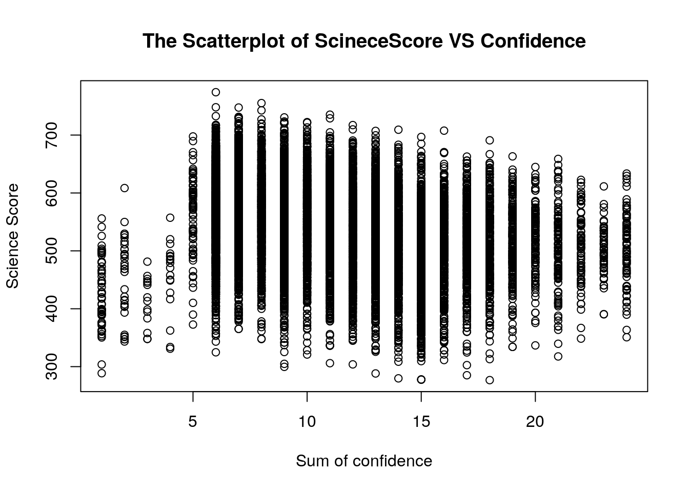
# Load the package. Don't forget to install the package before you use it.
# For install the package, type in: install.packages("Hmisc")
library(Hmisc)
# This time we want to find out what is the correlation between parents support and home stuff.
# First, we specify the data set first.
ParentSupport_VS_HomeStuff <- cbind(class_example$ParentSupport,class_example$Home)
# Calculate the Pearson correlation
rcorr(ParentSupport_VS_HomeStuff, type="pearson")
## [,1] [,2]
## [1,] 1.00 -0.11
## [2,] -0.11 1.00
##
## n
## [,1] [,2]
## [1,] 12908 12821
## [2,] 12821 12948
##
## P
## [,1] [,2]
## [1,] 0
## [2,] 0## [,1] [,2]
## [1,] 1.00 -0.12
## [2,] -0.12 1.00
##
## n
## [,1] [,2]
## [1,] 12908 12821
## [2,] 12821 12948
##
## P
## [,1] [,2]
## [1,] 0
## [2,] 0From the outcome table (the correlation matrix), we can see that the more parent support, the more home stuffs (r=-0.11,p=.00). It is because the higher values of sum of parent support indicate less support (see the TISS questionnaire).
Note*: Pearson & Spearman correlation could be also used on ordinal scales (ranking data).
# We take the Spearman_slide7.sav data for example
# Import the data first
Spearman_rank_example <- read_sav("Sperman_slide7.sav")
# Check the data set
Spearman_rank_example
## # A tibble: 10 x 4
## X Y Rank_X Rank_Y
## <dbl> <dbl> <dbl> <dbl>
## 1 12 36 4 8
## 2 16 25 7 4.5
## 3 10 35 2 7
## 4 11 38 3 9
## 5 15 24 6 3
## 6 9 40 1 10
## 7 21 18 10 1
## 8 14 33 5 6
## 9 17 25 8 4.5
## 10 19 22 9 2# Calculate the Pearson correlation
Result_Pearson <- rcorr(as.matrix(Spearman_rank_example),type="pearson")
Result_Pearson## X Y Rank_X Rank_Y
## X 1.00 -0.95 0.99 -0.94
## Y -0.95 1.00 -0.95 0.98
## Rank_X 0.99 -0.95 1.00 -0.92
## Rank_Y -0.94 0.98 -0.92 1.00
##
## n= 10
##
##
## P
## X Y Rank_X Rank_Y
## X 0e+00 0e+00 0e+00
## Y 0e+00 0e+00 0e+00
## Rank_X 0e+00 0e+00 1e-04
## Rank_Y 0e+00 0e+00 1e-04# Calculate the Spearman correlation
Result_Spearman <- rcorr(as.matrix(Spearman_rank_example),type="spearman")
Result_Spearman## X Y Rank_X Rank_Y
## X 1.00 -0.92 1.00 -0.92
## Y -0.92 1.00 -0.92 1.00
## Rank_X 1.00 -0.92 1.00 -0.92
## Rank_Y -0.92 1.00 -0.92 1.00
##
## n= 10
##
##
## P
## X Y Rank_X Rank_Y
## X 1e-04 0e+00 1e-04
## Y 1e-04 1e-04 0e+00
## Rank_X 0e+00 1e-04 1e-04
## Rank_Y 1e-04 0e+00 1e-044.2 Point Biserial Correlation & Phi Correlation
4.2.1 Point Biserial Correlation
The point biserial correlation coefficient is a correlation coefficient used when one variable (e.g. Y) is dichotomous; Y can either be “naturally” dichotomous, like whether a coin lands heads or tails, or an artificially dichotomized variable.
\[r_{P b i s}=\frac{\bar{Y}_{1}-\bar{Y}_{0}}{S_{Y}} \sqrt{\frac{n_{0} n_{1}}{N(N-1)}}\] Where \(n_{0}\) is the number of individuals coded 0 for variable X, \(n_{1}\) is the number of individuals coded 1 for variable X, and N is the total number of sample size \(n_{0}+n_{1}=N\).
# The point-biserial correlation is equivalent to calculating the Pearson correlation between a continuous and a dichotomous variable.
# You can just use the standard cor.test function in R, which will output the correlation, a 95% confidence interval, and an independent t-test with associated p-value.
cor.test(class_example$learning,class_example$gender)
##
## Pearson's product-moment correlation
##
## data: class_example$learning and class_example$gender
## t = 2.5608, df = 12878, p-value = 0.01045
## alternative hypothesis: true correlation is not equal to 0
## 95 percent confidence interval:
## 0.005292235 0.039815076
## sample estimates:
## cor
## 0.02256038The result above indicates that Girls (gender = 1) like to learn science less than boys (gender = 0) (r = .023, p = .01). It is because the higher values of sum of learning shows “they don’t like to learn science (see the TIMSS questionnaire).
4.2.2 Phi Correlation
The Phi Coefficient is a measure of association between two binary variables (i.e. living/dead, black/white, success/failure). The correlation is based on frequency counts. The equation could be denoted as:
\[\Phi=\frac{a d-b c}{\sqrt{(a+b)(c+d)(a+c)(b+d)}}\] Where a, b, c, & d represent the frequency of individuals.
# The phi coefficient is identical to the Pearson coefficient in the case of a 2 x 2 data set.
# We can still use the cor.test function to calculate the phi coefficient.
cor.test(class_example$gender,class_example$home_book)
##
## Pearson's product-moment correlation
##
## data: class_example$gender and class_example$home_book
## t = 9.697, df = 12898, p-value < 2.2e-16
## alternative hypothesis: true correlation is not equal to 0
## 95 percent confidence interval:
## 0.06791693 0.10218083
## sample estimates:
## cor
## 0.085074034.3 Partial and Semi-partial Correlation
The Partial correlation is the correlation of two variables while controlling for a third or more other variables. The partial correlation coefficient is a measure of the strength of the linear relationship between two variables after entirely controlling for the effects of other variables.
Semi-partial (or Part) Correlation: The semi-partial correlation coefficient is the correlation between all of Y and that part of X which is independent of Z. That is the effect of Z has been removed from X but not from Y.
# We can use the package 'ppcor' to calculate the partial and semi-partial correlation
library(ppcor)
# Both the calculation of the partial and semi-partial correlation are not allow the Missing Value, so we need prepare a clean data set without all the missing value.
uncleaned_data <- cbind(class_example$ScienceScore,class_example$engagement,class_example$learning)
cleaned_data <- na.omit(uncleaned_data)
names <- c("ScienceScore","Engagement","Learning")
colnames(cleaned_data) <- names
cleaned_data <- as.data.frame(cleaned_data)
# Calculate the correlation between science score and engagement while controlling the variable learning
pcor.test(cleaned_data$ScienceScore,cleaned_data$Engagement,cleaned_data$Learning,method="pearson")
## estimate p.value statistic n gp Method
## 1 -0.153554 1.257616e-68 -17.61272 12849 1 pearson# The outcome table indicates that the partial correlation between sum of engagement and ScienceScore after entirely controlling for the effects of sum of learning = -0.154.
# Similarly, the semi-partial correlations can be calculated with spcor() function.
spcor.test(cleaned_data$ScienceScore,cleaned_data$Engagement,cleaned_data$Learning,method="pearson")## estimate p.value statistic n gp Method
## 1 -0.1533073 2.072572e-68 -17.58374 12849 1 pearson