Chapter 6 Curvilinear Regression
6.1 Introduction to Curvilinear Regression
The curvilinear regression analysis can be used to determine if not-so-linear trends exist between X and Y.
A simple regression model extension for curved relations is the polynomial model. This is an example of curvilinear regression.
Hypothesis Test
A null hypothesis is there is no relationship between the X and Y variables when doing curvilinear regression.
Second null hypothesis is the increase in \(R^{2}\) is only as large as you would expect by chance.
As you add more parameters to an equation, it will always fit the data better. A quadratic and cubic equations will always have an equal or higher \(R^{2}\) than the linear. A cubic equation will usually have an equal or higher \(R^{2}\) than quadratic.
6.2 Descriptive Data Analysis
Just like any examples else, we need to prepare the data before we run the analysis.
## # A tibble: 6 x 8
##   anxiety perform anxiety_squared anxiety_third anxiety_mean anxiety_centered
##     <dbl>   <dbl>           <dbl>         <dbl>        <dbl>            <dbl>
## 1       1      12               1             1            4               -3
## 2       1      15               1             1            4               -3
## 3       2      26               4             8            4               -2
## 4       2      22               4             8            4               -2
## 5       3      42               9            27            4               -1
## 6       3      36               9            27            4               -1
## # … with 2 more variables: anxiety_centered_squared <dbl>,
## #   anxiety_centered_third <dbl>
# Plot a Scatterplot between IV and DV
plot(curvreg_data$anxiety,curvreg_data$perform, main="Scatterplot betwwen Anxiety and Performance",xlab="Anxiety",ylab="Performance")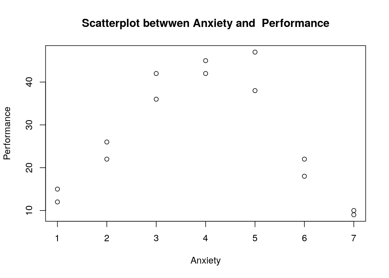
6.3 Run the Curvilinear Regression Model
6.3.1 Linear regression model
# Run a linear regression model by using lm() function
curvreg_lm <- lm(perform~anxiety,data=curvreg_data)
summary(curvreg_lm)
##
## Call:
## lm(formula = perform ~ anxiety, data = curvreg_data)
##
## Residuals:
## Min 1Q Median 3Q Max
## -17.196 -12.710 -3.429 13.277 20.161
##
## Coefficients:
## Estimate Std. Error t value Pr(>|t|)
## (Intercept) 29.7857 8.5704 3.475 0.00458 **
## anxiety -0.5893 1.9164 -0.307 0.76374
## ---
## Signif. codes: 0 '***' 0.001 '**' 0.01 '*' 0.05 '.' 0.1 ' ' 1
##
## Residual standard error: 14.34 on 12 degrees of freedom
## Multiple R-squared: 0.007818, Adjusted R-squared: -0.07486
## F-statistic: 0.09455 on 1 and 12 DF, p-value: 0.7637# Add fit lines
plot(perform~anxiety,data=curvreg_data)
abline(lm(perform~anxiety,data=curvreg_data))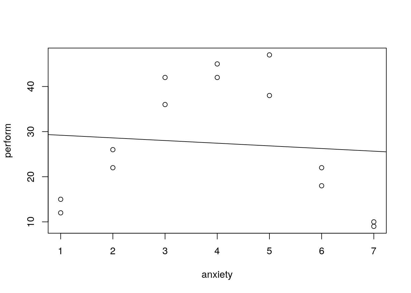
6.3.2 Quadratic regression model
The quadratic regression model is pretty similar with the multiple regression. The second independent variable here is the squared value of the 1st variable.
# Run a Quadratic regression model by using lm() function
curvreg_Quadm <- lm(perform~anxiety+anxiety_squared,data=curvreg_data)
summary(curvreg_Quadm)
##
## Call:
## lm(formula = perform ~ anxiety + anxiety_squared, data = curvreg_data)
##
## Residuals:
## Min 1Q Median 3Q Max
## -8.2500 -2.7946 0.5952 2.9405 9.3214
##
## Coefficients:
## Estimate Std. Error t value Pr(>|t|)
## (Intercept) -13.5714 5.5081 -2.464 0.0315 *
## anxiety 28.3155 3.1566 8.970 2.17e-06 ***
## anxiety_squared -3.6131 0.3856 -9.369 1.41e-06 ***
## ---
## Signif. codes: 0 '***' 0.001 '**' 0.01 '*' 0.05 '.' 0.1 ' ' 1
##
## Residual standard error: 4.998 on 11 degrees of freedom
## Multiple R-squared: 0.8895, Adjusted R-squared: 0.8694
## F-statistic: 44.28 on 2 and 11 DF, p-value: 5.473e-06Then we add a fit line
# load the ggplot package to use ggplot() function
library(ggplot2)
# Add fit lines
ggplot(curvreg_data, aes(x=anxiety, y=perform)) + geom_point()+stat_smooth(se=F, method='lm', formula=y~poly(x,2))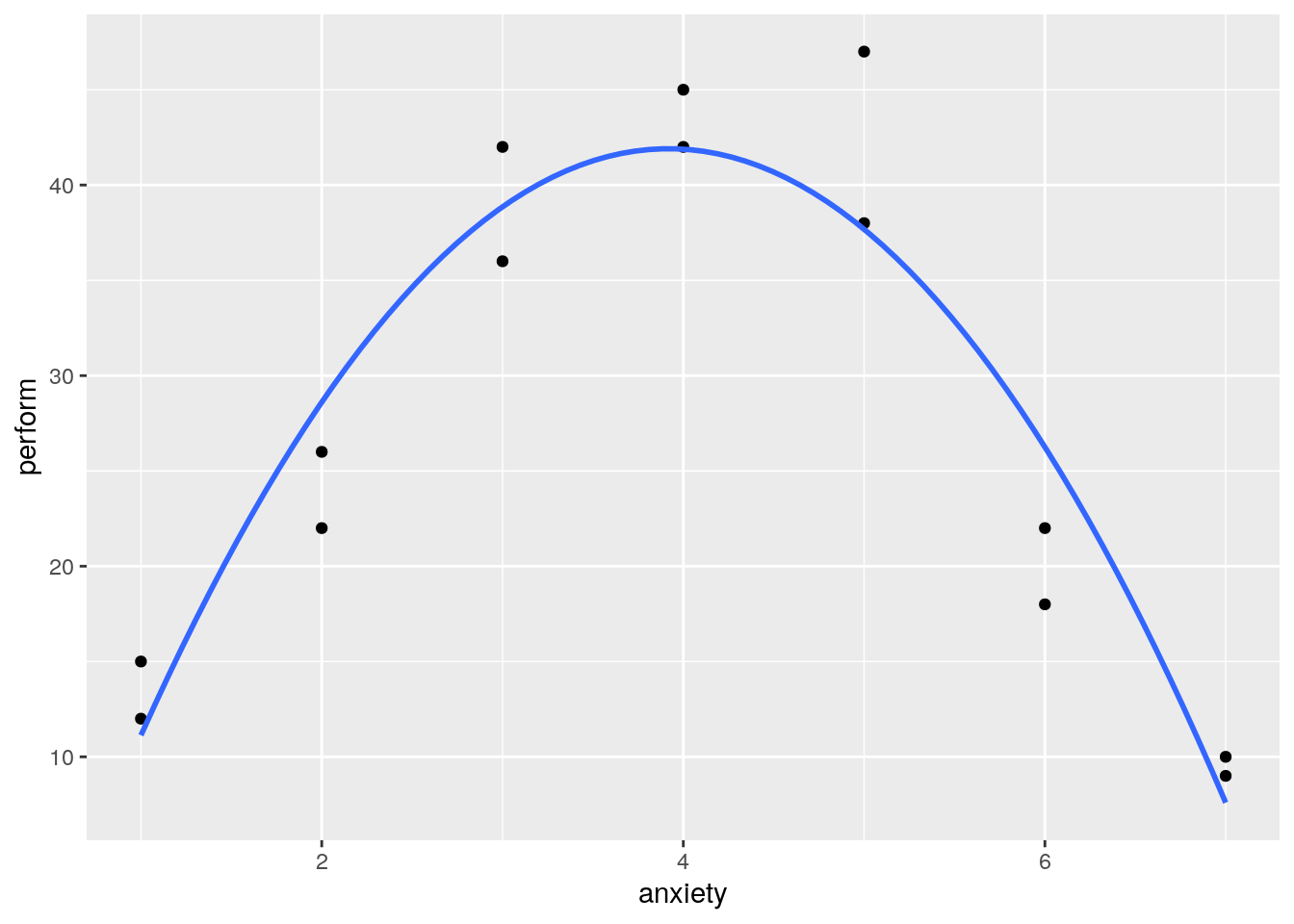
6.3.3 Cubic regression model
The cubic regression model is still pretty similar with the multiple regression. The third independent variable here is the cubic value of the 1st variable.
# Run a Cubic regression model by using lm() function
curvreg_cubreg <- lm(perform~anxiety+anxiety_squared+anxiety_third,data=curvreg_data)
summary(curvreg_cubreg)
##
## Call:
## lm(formula = perform ~ anxiety + anxiety_squared + anxiety_third,
## data = curvreg_data)
##
## Residuals:
## Min 1Q Median 3Q Max
## -8.8333 -2.2113 0.2024 3.0863 8.7381
##
## Coefficients:
## Estimate Std. Error t value Pr(>|t|)
## (Intercept) -10.07143 10.68184 -0.943 0.3680
## anxiety 24.32937 10.77739 2.257 0.0476 *
## anxiety_squared -2.44643 3.03087 -0.807 0.4383
## anxiety_third -0.09722 0.25035 -0.388 0.7059
## ---
## Signif. codes: 0 '***' 0.001 '**' 0.01 '*' 0.05 '.' 0.1 ' ' 1
##
## Residual standard error: 5.203 on 10 degrees of freedom
## Multiple R-squared: 0.8912, Adjusted R-squared: 0.8585
## F-statistic: 27.29 on 3 and 10 DF, p-value: 3.944e-05# Add fit lines
ggplot(curvreg_data, aes(x=anxiety, y=perform)) + geom_point()+stat_smooth(se=F, method='lm', formula=y~poly(x,3))
6.4 Model Comparison
From the previous section, we got three regression models, namely, linear, quadratic and cubic regression model.
# We can use the anova() function to compare three models
anova(curvreg_lm,curvreg_Quadm) # Compare linear with quadratic regression model
## Analysis of Variance Table
##
## Model 1: perform ~ anxiety
## Model 2: perform ~ anxiety + anxiety_squared
## Res.Df RSS Df Sum of Sq F Pr(>F)
## 1 12 2467.98
## 2 11 274.83 1 2193.2 87.779 1.412e-06 ***
## ---
## Signif. codes: 0 '***' 0.001 '**' 0.01 '*' 0.05 '.' 0.1 ' ' 1## Analysis of Variance Table
##
## Model 1: perform ~ anxiety + anxiety_squared
## Model 2: perform ~ anxiety + anxiety_squared + anxiety_third
## Res.Df RSS Df Sum of Sq F Pr(>F)
## 1 11 274.83
## 2 10 270.75 1 4.0833 0.1508 0.7059## Analysis of Variance Table
##
## Model 1: perform ~ anxiety
## Model 2: perform ~ anxiety + anxiety_squared + anxiety_third
## Res.Df RSS Df Sum of Sq F Pr(>F)
## 1 12 2467.98
## 2 10 270.75 2 2197.2 40.577 1.589e-05 ***
## ---
## Signif. codes: 0 '***' 0.001 '**' 0.01 '*' 0.05 '.' 0.1 ' ' 1We can also compare these three models in one shot.
## Analysis of Variance Table
##
## Model 1: perform ~ anxiety
## Model 2: perform ~ anxiety + anxiety_squared
## Model 3: perform ~ anxiety + anxiety_squared + anxiety_third
##   Res.Df     RSS Df Sum of Sq       F    Pr(>F)
## 1     12 2467.98
## 2     11  274.83  1   2193.15 81.0027 4.137e-06 ***
## 3     10  270.75  1      4.08  0.1508    0.7059
## ---
## Signif. codes:  0 '***' 0.001 '**' 0.01 '*' 0.05 '.' 0.1 ' ' 1
Since the Model 2 (Quadratic Regression Model) is statistically significant in its RSS, we will choose this model as our final model.