Chapter 9 Growth Model
9.1 Introduction to Growth Model
Growth models look at the rate of change of a variable over time, such as:
– Depression over 8 weeks of treatment
– Back pain over 10 weeks of physiotherapy
– Profits over months of the year
– Radioactive decay
In all cases we’re trying to see which model best describes the change over time: likelihood ratio test for nested models and model fit indices for non-nested models. Comparing to curvilinear regression which only has level 1, Growth model has more than one level.
9.2 R Lab: Growth Model
9.2.1 Organize Longitudinal Data: Long Format vs. Wide Format
For Long format/Univariate format:
Each person has multiple records
One for each measurement occasion
A period-level data set
Long format is used in a variety of statistical software such as SAS, HLM, SPSS, and R/Mplus
# Let's import the Long format dataset and take a glance
library(haven)
Data_LF <- read_sav("Honeymoon Period_long.sav")
# Preview the first 10 lines
head(Data_LF,10)
## # A tibble: 10 x 4
## Person Gender Time Life_Satisfaction
## <dbl> <dbl+lbl> <dbl> <dbl>
## 1 1 0 [Male] 0 6
## 2 1 0 [Male] 1 6
## 3 1 0 [Male] 2 5
## 4 1 0 [Male] 3 2
## 5 2 1 [Female] 0 7
## 6 2 1 [Female] 1 7
## 7 2 1 [Female] 2 8
## 8 2 1 [Female] 3 4
## 9 3 1 [Female] 0 4
## 10 3 1 [Female] 1 6## Person Gender Time Life_Satisfaction
## Min. : 1.00 Min. :0.0000 Min. :0.00 Min. : 1.000
## 1st Qu.: 32.00 1st Qu.:0.0000 1st Qu.:0.75 1st Qu.: 4.000
## Median : 66.00 Median :0.0000 Median :1.50 Median : 6.000
## Mean : 63.96 Mean :0.4957 Mean :1.50 Mean : 5.989
## 3rd Qu.: 95.00 3rd Qu.:1.0000 3rd Qu.:2.25 3rd Qu.: 8.000
## Max. :123.00 Max. :1.0000 Max. :3.00 Max. :10.000
## NA's :22We can find that in Life_satisfaction column, we got 22 missing data.
Then, we have the Wide format / Multivariate format, which is:
Each person has one record and multiple variables containing the data from each measurement
A Person-level data set
Wide format is used in SEM software such as Mplus, Lisrel, Mx, and Amos.
# Let's import the Wide format dataset and take a glance
library(haven)
Data_WF <- read_sav("Honeymoon Period_wide.sav")
# Preview the first 10 lines
head(Data_WF,10)
## # A tibble: 10 x 6
## Person Gender Life_Satisfacti… Life_Satisfacti… Life_Satisfacti…
## <dbl> <dbl+l> <dbl> <dbl> <dbl>
## 1 1 0 [Mal… 6 6 5
## 2 2 1 [Fem… 7 7 8
## 3 3 1 [Fem… 4 6 2
## 4 4 0 [Mal… 6 9 4
## 5 5 0 [Mal… 6 7 6
## 6 6 1 [Fem… 5 10 4
## 7 7 0 [Mal… 6 6 4
## 8 8 0 [Mal… 2 5 4
## 9 9 0 [Mal… 10 9 5
## 10 10 0 [Mal… 10 10 10
## # … with 1 more variable: Life_Satisfaction.3 <dbl>## Person Gender Life_Satisfaction.0 Life_Satisfaction.1
## Min. : 1.00 Min. :0.0000 Min. : 1.000 Min. : 2.000
## 1st Qu.: 32.50 1st Qu.:0.0000 1st Qu.: 5.000 1st Qu.: 5.500
## Median : 66.00 Median :0.0000 Median : 7.000 Median : 7.000
## Mean : 63.96 Mean :0.4957 Mean : 6.635 Mean : 7.026
## 3rd Qu.: 94.50 3rd Qu.:1.0000 3rd Qu.: 8.500 3rd Qu.: 9.000
## Max. :123.00 Max. :1.0000 Max. :10.000 Max. :10.000
##
## Life_Satisfaction.2 Life_Satisfaction.3
## Min. : 1.000 Min. :1.000
## 1st Qu.: 4.000 1st Qu.:2.000
## Median : 6.000 Median :4.000
## Mean : 5.788 Mean :4.189
## 3rd Qu.: 8.000 3rd Qu.:6.000
## Max. :10.000 Max. :9.000
## NA's :2 NA's :20It is easy to convert a longitudinal data set from one format to the other through R.
# We need "reshape" package to do the data transformation
library(reshape)
# We can use the cast() function to transform the long format data to wide format data
Data_LF2WF <- cast(Data_LF, Person+Gender~Time,value="Life_Satisfaction")
# To make our wide data exactly the same with the wide format, we need to correct the variable names.
# To do that, we need rename() function from the plyr package
library(plyr)
## ------------------------------------------------------------------------------## You have loaded plyr after dplyr - this is likely to cause problems.
## If you need functions from both plyr and dplyr, please load plyr first, then dplyr:
## library(plyr); library(dplyr)## ------------------------------------------------------------------------------##
## Attaching package: 'plyr'## The following objects are masked from 'package:reshape':
##
## rename, round_any## The following objects are masked from 'package:Hmisc':
##
## is.discrete, summarize## The following objects are masked from 'package:dplyr':
##
## arrange, count, desc, failwith, id, mutate, rename, summarise,
## summarizeReshaped_WF <- rename(Data_LF2WF,c("0"="Life_Satisfaction.0","1"="Life_Satisfaction.1","2"="Life_Satisfaction.2","3"="Life_Satisfaction.3"))
# Check the final version of reshaped dataset
head(Reshaped_WF,10)## Person Gender Life_Satisfaction.0 Life_Satisfaction.1 Life_Satisfaction.2
## 1 1 0 6 6 5
## 2 2 1 7 7 8
## 3 3 1 4 6 2
## 4 4 0 6 9 4
## 5 5 0 6 7 6
## 6 6 1 5 10 4
## 7 7 0 6 6 4
## 8 8 0 2 5 4
## 9 9 0 10 9 5
## 10 10 0 10 10 10
## Life_Satisfaction.3
## 1 2
## 2 4
## 3 2
## 4 1
## 5 6
## 6 2
## 7 2
## 8 NA
## 9 6
## 10 9# Also, we can use the melt() function to transform the wide format data to long format data
Data_WF2LF <- melt(as.data.frame(Data_WF), id=c("Person","Gender"),Measured=c("Life_Satisfaction.0", "Life_Satisfaction.1", "Life_Satisfaction.2", "Life_Satisfaction.3"))
# To make our long data exactly the same with the long format, we need to set the levels of variable, and correct the variable name of "value"
Reshaped_LF <- rename(Data_WF2LF,c("value"="Life_Satisfaction","variable"="Time"))
# Wait, the level names of the variable is still not right!
# We can use the levels() function to change the level names of the variable.
levels(Reshaped_LF$Time) <- c(0, 1, 2, 3)
# Check the final version of reshaped dataset
head(Reshaped_LF,10)## Person Gender Time Life_Satisfaction
## 1 1 0 0 6
## 2 2 1 0 7
## 3 3 1 0 4
## 4 4 0 0 6
## 5 5 0 0 6
## 6 6 1 0 5
## 7 7 0 0 6
## 8 8 0 0 2
## 9 9 0 0 10
## 10 10 0 0 109.2.2 An Example of Honeymoon Data
9.2.2.1 Load the data
# Load the data into the R first
HPL <- read_sav("Honeymoon Period_long.sav")
# Check the data structure
str(HPL)
## tibble [460 × 4] (S3: tbl_df/tbl/data.frame)
## $ Person : num [1:460] 1 1 1 1 2 2 2 2 3 3 ...
## ..- attr(*, "label")= chr "Participant Number"
## ..- attr(*, "format.spss")= chr "F2.0"
## $ Gender : dbl+lbl [1:460] 0, 0, 0, 0, 1, 1, 1, 1, 1, 1, 1, 1, 0, 0, 0, 0, 0, 0, ...
## ..@ label : chr "Gender"
## ..@ format.spss : chr "F8.0"
## ..@ display_width: int 10
## ..@ labels : Named num [1:2] 0 1
## .. ..- attr(*, "names")= chr [1:2] "Male" "Female"
## $ Time : num [1:460] 0 1 2 3 0 1 2 3 0 1 ...
## ..- attr(*, "label")= chr "Time"
## ..- attr(*, "format.spss")= chr "F4.0"
## $ Life_Satisfaction: num [1:460] 6 6 5 2 7 7 8 4 4 6 ...
## ..- attr(*, "label")= chr "Life Satisfaction"
## ..- attr(*, "format.spss")= chr "F8.0"
## ..- attr(*, "display_width")= int 13## Person Gender Time Life_Satisfaction
## Min. : 1.00 Min. :0.0000 Min. :0.00 Min. : 1.000
## 1st Qu.: 32.00 1st Qu.:0.0000 1st Qu.:0.75 1st Qu.: 4.000
## Median : 66.00 Median :0.0000 Median :1.50 Median : 6.000
## Mean : 63.96 Mean :0.4957 Mean :1.50 Mean : 5.989
## 3rd Qu.: 95.00 3rd Qu.:1.0000 3rd Qu.:2.25 3rd Qu.: 8.000
## Max. :123.00 Max. :1.0000 Max. :3.00 Max. :10.000
## NA's :22Variables included in the data set
• Speed Dating Event
– After a speed-dating event, data were collected on all people who ended up in a relationship with the person that they met on the speed-dating night.
– None of the people measured were in the same relationship.
• Satisfaction_Baseline
– A 10-point scale (0= completely dissatisfied,10 = completely satisfied)
• Satisfaction_6_Months
– Life satisfaction at 6 months(0-10)
• Satisfaction_12_Months
– Life satisfaction at 12 months(0-10)
• Satisfaction_18_Months
– Life satisfaction at 18months(0-10)
• Gender
– 0=male,1=female
9.2.2.2 Plot the data
We can build a Scatter plot to overview the data.
# We need "ggplot2" package to plot
library(ggplot2)
# Run a Scatter plot
ggplot(HPL,aes(x=Time, y=Life_Satisfaction))+geom_point()+geom_smooth()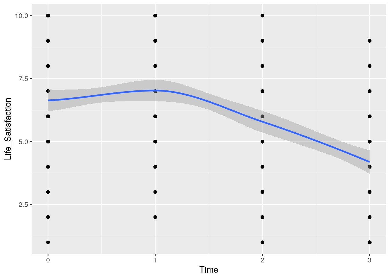
9.2.2.3 Set a baseline model
Set a baseline model predicting life satisfaction from only the intercept.
# Load the "nlme" package to run the growth model
library(nlme)
# Fit a basic model
intercept <-gls(Life_Satisfaction ~ 1, data = HPL, method = "ML", na.action = na.exclude)
summary(intercept)
## Generalized least squares fit by maximum likelihood
## Model: Life_Satisfaction ~ 1
## Data: HPL
## AIC BIC logLik
## 2064.053 2072.217 -1030.026
##
## Coefficients:
## Value Std.Error t-value p-value
## (Intercept) 5.988584 0.1215722 49.25948 0
##
## Standardized residuals:
## Min Q1 Med Q3 Max
## -1.962918615 -0.782472363 0.004491805 0.791455972 1.578420140
##
## Residual standard error: 2.541412
## Degrees of freedom: 438 total; 437 residualFrom the result that we can tell the life satisfaction in this group of people are significantly different with each other (one sample t-test,t=49.26,p<0.01).
9.2.2.4 A model with random intercepts across people (randomIntercept)
# Next, we need to fit the same model, but this time allowing the intercepts to vary across contexts (in this case we want them to vary across people).
randomIntercept <-lme(Life_Satisfaction ~ 1, data = HPL,
            random = ~1|Person, method = "ML",  na.action = na.exclude, control =
            list(opt="optim"))
Note that we have asked R to create an object called intercept, and we have specified that Life_Satisfaction is the outcome variable and that it is predicted from only the intercept (the ‘~1’ in the function).
The rest of the function specifies the data (data = HPL) and how to estimate the model (method = “ML”).
Note that there is a new option that we have not encountered before: control = list(opt=“optim”). This option changes the optimizer that R uses to estimate the model.
9.2.2.5 A model with time as a predictor of life satisfaction and random intercepts across people (timeRI)
# Adding in time as a fixed effect: timeRandomIntercept
timeRI<-update(randomIntercept, .~. + Time)
# Have a look at the new model
summary(timeRI)
## Linear mixed-effects model fit by maximum likelihood
## Data: HPL
## AIC BIC logLik
## 1871.728 1888.057 -931.8642
##
## Random effects:
## Formula: ~1 | Person
## (Intercept) Residual
## StdDev: 1.749013 1.629312
##
## Fixed effects: Life_Satisfaction ~ Time
## Value Std.Error DF t-value p-value
## (Intercept) 7.208838 0.20780657 322 34.69014 0
## Time -0.877218 0.07191951 322 -12.19722 0
## Correlation:
## (Intr)
## Time -0.488
##
## Standardized Within-Group Residuals:
## Min Q1 Med Q3 Max
## -2.25890447 -0.66898141 0.06207131 0.52437091 2.80332402
##
## Number of Observations: 438
## Number of Groups: 115This variable in our data set is the index variable (Time), which specifies whether the life satisfaction score was recorded at baseline (0), 6 months (1), 12 months (2) or 18 months (3).
In the previous example we built up our models individually using the lme() function; however, for this example our models have a lot of options (method = “ML”, na.action = na.exclude, control = list(opt=“optim”)), which we must specify in each new model. This typing would be tedious, so we will use the update() function to retain everything from a previous model (including options such as the method, how to deal with missing cases, and the optimization method) but add things to it (R’s Souls’ Tip 19.3).
This command creates a new object in R called timeRI. The first part of the parenthesis tells R which model to update (in this case we have updated randomIntercept). The remainder tells R how to update this model: .~. simply means ‘keep the previous outcome and all of the previous predictors’ and + Time means ‘add Time as a predictor’. If you want to have a look at the new model you can use summary(timeRI).
9.2.2.6 A model with time as a predictor, a random effect of time over people and random intercepts (timeRS)
At the moment, the random part of the model is specified as random = ~1|Person, which means that intercepts (~1) vary across people (Person). If we want slopes to vary across people as well, then we’re saying that the effect of Time is different in different people.
This is a standard growth model scenario: the rate of development or growth over time differs within entities (in this case people, but it could be companies, mice, states, hospitals, schools, geographical areas, etc.).
As such, we want to update the random part of the model to be random = ~Time|Person, which means that intercepts and the effect of time (~Time) vary across people (Person).
# Introducing random slopes
timeRS<-update(timeRI, random = ~Time|Person)
# Take a look
summary(timeRS)
## Linear mixed-effects model fit by maximum likelihood
## Data: HPL
## AIC BIC logLik
## 1874.626 1899.12 -931.3131
##
## Random effects:
## Formula: ~Time | Person
## Structure: General positive-definite, Log-Cholesky parametrization
## StdDev Corr
## (Intercept) 1.8617835 (Intr)
## Time 0.3035857 -0.361
## Residual 1.5855237
##
## Fixed effects: Life_Satisfaction ~ Time
## Value Std.Error DF t-value p-value
## (Intercept) 7.207838 0.21420441 322 33.64934 0
## Time -0.875734 0.07578349 322 -11.55574 0
## Correlation:
## (Intr)
## Time -0.537
##
## Standardized Within-Group Residuals:
## Min Q1 Med Q3 Max
## -2.06051254 -0.68153140 0.02527726 0.52380774 2.63779515
##
## Number of Observations: 438
## Number of Groups: 115We use the update() function to create a new model (called timeRS) which is identical to the previous model (timeRI) but updates the random part of the model to be random = ~Time|Person.
9.2.2.7 A model with time as a predictor, random effects of time across people, a random effect of intercepts across people, and a first-order autoregressive covariance structure (ARModel)
Now we have a basic random effects model, we can introduce a term that models the covariance structure or errors.We do this by using the option correlation = x, in which x is one of several pre-defined covariance structures.
# Modelling the covariance structure
ARModel<-update(timeRS, correlation = corAR1(0, form = ~Time|Person))
# Take a look at the new model
summary(ARModel)
## Linear mixed-effects model fit by maximum likelihood
## Data: HPL
## AIC BIC logLik
## 1872.891 1901.466 -929.4453
##
## Random effects:
## Formula: ~Time | Person
## Structure: General positive-definite, Log-Cholesky parametrization
## StdDev Corr
## (Intercept) 1.62767553 (Intr)
## Time 0.04782877 -0.062
## Residual 1.74812486
##
## Correlation Structure: AR(1)
## Formula: ~Time | Person
## Parameter estimate(s):
## Phi
## 0.2147812
## Fixed effects: Life_Satisfaction ~ Time
## Value Std.Error DF t-value p-value
## (Intercept) 7.131470 0.21260192 322 33.54377 0
## Time -0.870087 0.07929275 322 -10.97310 0
## Correlation:
## (Intr)
## Time -0.527
##
## Standardized Within-Group Residuals:
## Min Q1 Med Q3 Max
## -2.08400991 -0.62083911 0.06392492 0.59512953 2.49161500
##
## Number of Observations: 438
## Number of Groups: 115Note that we have used correlation = corAR1(0, form = ~Time|Person). We could have used the default setting, which would be to use correlation = corAR1(), but this would include only the random intercept (it would be the same as specifying correlation = corAR1(0, form = ~1|Person).
9.2.2.8 Compare the models
So far we have created five models:
A baseline model predicting life satisfaction from only the intercept (interceptOnly);
A model with random intercepts across people (randomIntercept);
A model with time as a predictor of life satisfaction and random inter- cepts across people (timeRI);
A model with time as a predictor, a random effect of time over people and random intercepts (timeRS);
A model with time as a predictor, random effects of time across people, a random effect of intercepts across people, and a first-order autoregressive covariance structure (ARModel).
# Let's take a look at how these model fit the data.
# We can compare all five models by using anova() function.
anova(intercept, randomIntercept, timeRI, timeRS, ARModel)## Model df AIC BIC logLik Test L.Ratio p-value
## intercept 1 2 2064.053 2072.217 -1030.0263
## randomIntercept 2 3 1991.396 2003.642 -992.6978 1 vs 2 74.65704 <.0001
## timeRI 3 4 1871.728 1888.057 -931.8642 2 vs 3 121.66714 <.0001
## timeRS 4 6 1874.626 1899.120 -931.3131 3 vs 4 1.10224 0.5763
## ARModel 5 7 1872.891 1901.466 -929.4453 4 vs 5 3.73564 0.0533The resulting output shows that adding a random intercept significantly improved the fit of the model, \(χ^2\)(1) = 74.66, p < .0001. Similarly, adding the fixed effect of time to the model significantly improved the fit compared to the previous model, \(χ^2\)(1) = 121.67, p < .0001. However, adding a random slope for the effect of time across participants did not significantly improve the model, \(χ^2\)(2) = 1.10, p = .576. Finally, adding a first-order autoregressive covariance structure did more or less significantly improve the model, \(χ^2\) (1) = 3.74, p = .053. Note that for each model the degrees of freedom change by 1 because we have added only a single parameter; this change in degrees of freedom is used for the log-likelihood test.
## Linear mixed-effects model fit by maximum likelihood
##  Data: HPL
##        AIC      BIC    logLik
##   1872.891 1901.466 -929.4453
##
## Random effects:
##  Formula: ~Time | Person
##  Structure: General positive-definite, Log-Cholesky parametrization
##             StdDev     Corr
## (Intercept) 1.62767553 (Intr)
## Time        0.04782877 -0.062
## Residual    1.74812486
##
## Correlation Structure: AR(1)
##  Formula: ~Time | Person
##  Parameter estimate(s):
##       Phi
## 0.2147812
## Fixed effects: Life_Satisfaction ~ Time
##                 Value  Std.Error  DF   t-value p-value
## (Intercept)  7.131470 0.21260192 322  33.54377       0
## Time        -0.870087 0.07929275 322 -10.97310       0
##  Correlation:
##      (Intr)
## Time -0.527
##
## Standardized Within-Group Residuals:
##         Min          Q1         Med          Q3         Max
## -2.08400991 -0.62083911  0.06392492  0.59512953  2.49161500
##
## Number of Observations: 438
## Number of Groups: 115## Person = pdLogChol(Time)
## Variance StdDev Corr
## (Intercept) 2.649327640 1.62767553 (Intr)
## Time 0.002287591 0.04782877 -0.062
## Residual 3.055940530 1.74812486Intepretation:
The resulting model summary and Output 19.20 shows the 95% confidence intervals. The effect of time, b = -0.87 (-1.03, -0.71), t(322) = -10.97, p < .001, was highly significant, indicating that life satisfaction significantly changed over the 18 month period.
In addition, the standard deviation of intercepts was 1.62 (1.31, 2.02), and for the effect of time across people (slopes) was 0.05 (0.00, 41.83). Neither of the confidence intervals crosses zero, implying that this variance in slopes and intercepts was significant.
Note that in the case of the slopes, this finding contradicts the results of the log-likelihood statistic, which implied that adding random slopes did not significantly improve the model.
The approximate confidence interval for slopes is very wide and not symmetrical, which implies that we might be wise to give more weight to the log-likelihood.
9.2.3 Adding higher-order polynomials
9.2.3.1 Why we meed a higher-order polynomials?
In the previous model, we have seen that the main effect of time is significant. This main effect is the linear trend of time.
However, the plot above show a more curvilinear change over time (satisfaction first increases from baseline to 6 months before declining after 6 months).
To capture this trend we would need to add a quadratic or perhaps even cubic trend. We could simply create new predictor variables in our dataframe that are time multiplied by itself (time2) or time multiplied by itself twice (time3). We could then enter these new variables as predictors into the model.
9.2.3.2 Fit a Quadratic Model on Time
# Run a quadratic model on time
timeQuadratic<-update(ARModel, .~. + I(Time^2))
# Take a look
summary(timeQuadratic)
## Linear mixed-effects model fit by maximum likelihood
## Data: HPL
## AIC BIC logLik
## 1817.544 1850.202 -900.772
##
## Random effects:
## Formula: ~Time | Person
## Structure: General positive-definite, Log-Cholesky parametrization
## StdDev Corr
## (Intercept) 1.8930039 (Intr)
## Time 0.4182303 -0.341
## Residual 1.4465061
##
## Correlation Structure: AR(1)
## Formula: ~Time | Person
## Parameter estimate(s):
## Phi
## 0.1103841
## Fixed effects: Life_Satisfaction ~ Time + I(Time^2)
## Value Std.Error DF t-value p-value
## (Intercept) 6.676533 0.22174444 321 30.109135 0e+00
## Time 0.758773 0.21233264 321 3.573512 4e-04
## I(Time^2) -0.561659 0.06801598 321 -8.257756 0e+00
## Correlation:
## (Intr) Time
## Time -0.431
## I(Time^2) 0.271 -0.933
##
## Standardized Within-Group Residuals:
## Min Q1 Med Q3 Max
## -2.70821970 -0.52734402 -0.03624493 0.50891314 2.81358324
##
## Number of Observations: 438
## Number of Groups: 115We can create a model (timeCubic) that adds a cubic term in exactly the same way as for the quadratic trend. This time, we update the quadratic model (timeQuadratic) so that it includes time3, which is done the same as for the quadratic trend except that we specify time cubed rather than squared, ‘I(Time^3)’.
9.2.3.3 Fit a Cubic Model on Time
## Linear mixed-effects model fit by maximum likelihood
##  Data: HPL
##        AIC      BIC    logLik
##   1816.162 1852.902 -899.0808
##
## Random effects:
##  Formula: ~Time | Person
##  Structure: General positive-definite, Log-Cholesky parametrization
##             StdDev    Corr
## (Intercept) 1.8826725 (Intr)
## Time        0.4051351 -0.346
## Residual    1.4572374
##
## Correlation Structure: AR(1)
##  Formula: ~Time | Person
##  Parameter estimate(s):
##       Phi
## 0.1326346
## Fixed effects: Life_Satisfaction ~ Time + I(Time^2) + I(Time^3)
##                 Value Std.Error  DF   t-value p-value
## (Intercept)  6.634783 0.2230273 320 29.748744  0.0000
## Time         1.546635 0.4772221 320  3.240913  0.0013
## I(Time^2)   -1.326426 0.4209411 320 -3.151098  0.0018
## I(Time^3)    0.171096 0.0929297 320  1.841131  0.0665
##  Correlation:
##           (Intr) Time   I(T^2)
## Time      -0.278
## I(Time^2)  0.139 -0.951
## I(Time^3) -0.098  0.896 -0.987
##
## Standardized Within-Group Residuals:
##         Min          Q1         Med          Q3         Max
## -2.58597365 -0.54411056 -0.04373592  0.50525444  2.78413461
##
## Number of Observations: 438
## Number of Groups: 115
We can compare these two new models with the model taht included only the linear trend of time (ARModel) using the anova() function.
# Compare the high-order polynomial model with the linear trend model
anova(ARModel,timeQuadratic,timeCubic)
## Model df AIC BIC logLik Test L.Ratio p-value
## ARModel 1 7 1872.891 1901.466 -929.4453
## timeQuadratic 2 8 1817.544 1850.202 -900.7720 1 vs 2 57.34661 <.0001
## timeCubic 3 9 1816.161 1852.901 -899.0808 2 vs 3 3.38245 0.0659## Approximate 95% confidence intervals
##
## Fixed effects:
## lower est. upper
## (Intercept) 6.2417739 6.6765333 7.111293
## Time 0.3424670 0.7587732 1.175079
## I(Time^2) -0.6950137 -0.5616594 -0.428305
## attr(,"label")
## [1] "Fixed effects:"
##
## Random Effects:
## Level: Person
## lower est. upper
## sd((Intercept)) 1.5062500 1.8930039 2.37906296
## sd(Time) 0.1884318 0.4182303 0.92827535
## cor((Intercept),Time) -0.6613084 -0.3410199 0.08444142
##
## Correlation structure:
## lower est. upper
## Phi -0.2025314 0.1103841 0.4028464
## attr(,"label")
## [1] "Correlation structure:"
##
## Within-group standard error:
## lower est. upper
## 1.173614 1.446506 1.782852## Approximate 95% confidence intervals
##
## Fixed effects:
## lower est. upper
## (Intercept) 6.1980057 6.6347826 7.0715595
## Time 0.6120429 1.5466350 2.4812271
## I(Time^2) -2.1507978 -1.3264264 -0.5020551
## I(Time^3) -0.0108979 0.1710958 0.3530895
## attr(,"label")
## [1] "Fixed effects:"
##
## Random Effects:
## Level: Person
## lower est. upper
## sd((Intercept)) 1.4775551 1.8826725 2.39886548
## sd(Time) 0.1656451 0.4051351 0.99088027
## cor((Intercept),Time) -0.6750383 -0.3461486 0.09750834
##
## Correlation structure:
## lower est. upper
## Phi -0.2070036 0.1326346 0.4437416
## attr(,"label")
## [1] "Correlation structure:"
##
## Within-group standard error:
## lower est. upper
## 1.159362 1.457237 1.831647Interpretation
From the model comparison, it is clear from this that adding the quadratic term to the model significantly improves the fit, χ2(1) = 57.35, p < .0001; how- ever, adding in the cubic trend does not, χ2(1) = 3.38, p = .066.
Looking at the summary of the final model, the fixed effects and the confidence intervals tell us that the linear, b = 1.55 (0.61, 2.48), t(320) = 3.24, p < .01, and quadratic, b = -1.33 (-2.15, -0.50), t(320) = -3.15, p < .01, both significantly described the pattern of the data over time; however, the cubic trend was not significant, b = 0.17 (-0.01, 0.35), t(320) = 1.84, p > .05. This confirms what we already know from comparing the fit of successive models.
This reflects the initial increase in life satisfaction 6 months after finding a new partner but a subsequent reduction in life satisfaction at 12 and 18 months after the start of the relationship.
It’s worth remembering that this quadratic trend is only an approximation: if it were completely accurate then we would predict from the model that couples who had been together for 10 years would have negative life satisfaction, which is impossible given the scale we used to measure it.
The outputs for the final model also tell us about the random parameters in the model. First of all, the standard deviation of the random intercepts was 1.88 (1.49, 2.39). The fact that the 95% confidence interval doesn’t cross zero suggests that we were correct to assume that life satisfaction at baseline varied significantly across people.
Also, the variance of slope of time varied significantly across people, SD = 0.41 (0.17, 0.96). The confidence interval again does not cross zero, suggesting that the change in life satisfaction over time varied significantly across people too.
Finally, the correlation between the slopes and intercepts, -0.35 (-0.67, 0.10) suggests that as intercepts increased, the slope decreased (although the confidence interval crosses zero so this trend is not significant).
9.3 Supplementary Learning Materials
Field, A. (2013). Discovering statistics using IBM SPSS statistics (4th ed.). Los Angeles, CA: Sage Publications.
Bickel, R. (2007). Multilevel Analysis for Applied Research: It’s just regression. NY: Guilford.
Raudenbush, S. W. & Bryk, A. S. (2002). Hierarchical Linear Models: Applications and Data Analysis Methods (2nd ed.). CA: Sage Publications
Using R and lme/lmer to fit different two- and three- level longitudinal models: Link
Linear Growth Model: Link
Analysing Longitudinal Data: Multilevel Growth Models: Link