Chapter 10 Binary Logistic Regression
10.1 Introduction
Logistic regression is a technique used when the dependent variable is categorical (or nominal). Examples: 1) Consumers make a decision to buy or not to buy, 2) a product may pass or fail quality control, 3) there are good or poor credit risks, and 4) employee may be promoted or not.
Binary logistic regression - determines the impact of multiple independent variables presented simultaneously to predict membership of one or other of the two dependent variable categories.
Since the dependent variable is dichotomous we cannot predict a numerical value for it using logistic regression so the usual regression least squares deviations criteria for best fit approach of minimizing error around the line of best fit is inappropriate (It’s impossible to calculate deviations using binary variables!).
Instead, logistic regression employs binomial probability theory in which there are only two values to predict: that probability (p) is 1 rather than 0, i.e. the event/person belongs to one group rather than the other.
Logistic regression forms a best fitting equation or function using the maximum likelihood (ML) method, which maximizes the probability of classifying the observed data into the appropriate category given the regression coefficients.
Like multiple regression, logistic regression provides a coefficient ‘b’, which measures each independent variable’s partial contribution to variations in the dependent variable.
The goal is to correctly predict the category of outcome for individual cases using the most parsimonious model.
To accomplish this goal, a model (i.e. an equation) is created that includes all predictor variables that are useful in predicting the response variable.
10.2 The Purpose of Binary Logistic Regression
- The logistic regression predicts group membership
Since logistic regression calculates the probability of success over the probability of failure, the results of the analysis are in the form of an odds ratio.
Logistic regression determines the impact of multiple independent variables presented simultaneously to predict membership of one or other of the two dependent variable categories.
- The logistic regression also provides the relationships and strengths among the variables ## Assumptions of (Binary) Logistic Regression
Logistic regression does not assume a linear relationship between the dependent and independent variables.
- Logistic regression assumes linearity of independent variables and log odds of dependent variable.
The independent variables need not be interval, nor normally distributed, nor linearly related, nor of equal variance within each group
- Homoscedasticity is not required. The error terms (residuals) do not need to be normally distributed.
The dependent variable in logistic regression is not measured on an interval or ratio scale.
- The dependent variable must be a dichotomous ( 2 categories) for the binary logistic regression.
The categories (groups) as a dependent variable must be mutually exclusive and exhaustive; a case can only be in one group and every case must be a member of one of the groups.
Larger samples are needed than for linear regression because maximum coefficients using a ML method are large sample estimates. A minimum of 50 cases per predictor is recommended (Field, 2013)
Hosmer, Lemeshow, and Sturdivant (2013) suggest a minimum sample of 10 observations per independent variable in the model, but caution that 20 observations per variable should be sought if possible.
Leblanc and Fitzgerald (2000) suggest a minimum of 30 observations per independent variable.
10.3 Log Transformation
The log transformation is, arguably, the most popular among the different types of transformations used to transform skewed data to approximately conform to normality.
- Log transformations and sq. root transformations moved skewed distributions closer to normality. So what we are about to do is common.
This log transformation of the p values to a log distribution enables us to create a link with the normal regression equation. The log distribution (or logistic transformation of p) is also called the logit of p or logit(p).
In logistic regression, a logistic transformation of the odds (referred to as logit) serves as the depending variable:
\[\log (o d d s)=\operatorname{logit}(P)=\ln \left(\frac{P}{1-P}\right)\] If we take the above dependent variable and add a regression equation for the independent variables, we get a logistic regression:
\[\ logit(p)=a+b_{1} x_{1}+b_{2} x_{2}+b_{3} x_{3}+\ldots\] As in least-squares regression, the relationship between the logit(P) and X is assumed to be linear.
10.4 Equation
\[P=\frac{\exp \left(a+b_{1} x_{1}+b_{2} x_{2}+b_{3} x_{3}+\ldots\right)}{1+\exp \left(a+b_{1} x_{1}+b_{2} x_{2}+b_{3} x_{3}+\ldots\right)}\] In the equation above: P can be calculated with the following formula
where:
P = the probability that a case is in a particular category,
exp = the exponential function (approx. 2.72),
a = the constant (or intercept) of the equation and,
b = the coefficient (or slope) of the predictor variables.
10.5 Hypothesis Test
In logistic regression, hypotheses are of interest:
the null hypothesis, which is when all the coefficients in the regression equation take the value zero, and
the alternate hypothesis that the model currently under consideration is accurate and differs significantly from the null of zero, i.e. gives significantly better than the chance or random prediction level of the null hypothesis.
10.6 Likelihood Ratio Test for Nested Models
The likelihood ratio test is based on -2LL ratio. It is a test of the significance of the difference between the likelihood ratio (-2LL) for the researcher’s model with predictors (called model chi square) minus the likelihood ratio for baseline model with only a constant in it.
Significance at the .05 level or lower means the researcher’s model with the predictors is significantly different from the one with the constant only (all ‘b’ coefficients being zero). It measures the improvement in fit that the explanatory variables make compared to the null model.
Chi square is used to assess significance of this ratio.
10.7 R Lab: Running Binary Logistic Regression Model
10.7.1 Data Explanations ((Data set: class.sav))
A researcher is interested in how variables, such as GRE (Graduate Record Exam scores), GPA (grade point average) and prestige of the undergraduate institution, effect admission into graduate school. The response variable, admit/don’t admit, is a binary variable.
This dataset has a binary response (outcome, dependent) variable called admit, which is equal to 1 if the individual was admitted to graduate school, and 0 otherwise.
There are three predictor variables: GRE, GPA, and rank. We will treat the variables GRE and GPA as continuous. The variable rank takes on the values 1 through 4. Institutions with a rank of 1 have the highest prestige, while those with a rank of 4 have the lowest.
10.7.2 Explore the data
## # A tibble: 6 x 5
##           admit        admit1   gre   gpa  rank
##       <dbl+lbl>     <dbl+lbl> <dbl> <dbl> <dbl>
## 1 0 [not admit] 1 [not admit]   380  3.61     3
## 2 1 [admit]     2 [admit]       660  3.67     3
## 3 1 [admit]     2 [admit]       800  4        1
## 4 1 [admit]     2 [admit]       640  3.19     4
## 5 0 [not admit] 1 [not admit]   520  2.93     4
## 6 1 [admit]     2 [admit]       760  3        2
This dataset has a binary response (outcome, dependent) variable called admit. There are three predictor variables: gre, gpa and rank. We will treat the variables gre and gpa as continuous. The variable rank takes on the values 1 through 4. Institutions with a rank of 1 have the highest prestige, while those with a rank of 4 have the lowest. We can get basic descriptives for the entire data set by using summary. To get the standard deviations, we use sapply to apply the sd function to each variable in the dataset.
##      admit            admit1           gre             gpa
##  Min.   :0.0000   Min.   :1.000   Min.   :220.0   Min.   :2.260
##  1st Qu.:0.0000   1st Qu.:1.000   1st Qu.:520.0   1st Qu.:3.130
##  Median :0.0000   Median :1.000   Median :580.0   Median :3.395
##  Mean   :0.3175   Mean   :1.317   Mean   :587.7   Mean   :3.390
##  3rd Qu.:1.0000   3rd Qu.:2.000   3rd Qu.:660.0   3rd Qu.:3.670
##  Max.   :1.0000   Max.   :2.000   Max.   :800.0   Max.   :4.000
##       rank
##  Min.   :1.000
##  1st Qu.:2.000
##  Median :2.000
##  Mean   :2.485
##  3rd Qu.:3.000
## Max. :4.000## admit admit1 gre gpa rank
## 0.4660867 0.4660867 115.5165364 0.3805668 0.9444602##
## 0 1
## 273 127##
## 1 2 3 4
## 61 151 121 67# To see the crosstable, we need CrossTable function from gmodels package
library(gmodels)
# Build a crosstable between admit and rank
CrossTable(class$admit, class$rank)##
##
## Cell Contents
## |-------------------------|
## | N |
## | Chi-square contribution |
## | N / Row Total |
## | N / Col Total |
## | N / Table Total |
## |-------------------------|
##
##
## Total Observations in Table: 400
##
##
## | class$rank
## class$admit | 1 | 2 | 3 | 4 | Row Total |
## -------------|-----------|-----------|-----------|-----------|-----------|
## 0 | 28 | 97 | 93 | 55 | 273 |
## | 4.464 | 0.356 | 1.314 | 1.880 | |
## | 0.103 | 0.355 | 0.341 | 0.201 | 0.682 |
## | 0.459 | 0.642 | 0.769 | 0.821 | |
## | 0.070 | 0.242 | 0.233 | 0.138 | |
## -------------|-----------|-----------|-----------|-----------|-----------|
## 1 | 33 | 54 | 28 | 12 | 127 |
## | 9.596 | 0.765 | 2.825 | 4.042 | |
## | 0.260 | 0.425 | 0.220 | 0.094 | 0.318 |
## | 0.541 | 0.358 | 0.231 | 0.179 | |
## | 0.083 | 0.135 | 0.070 | 0.030 | |
## -------------|-----------|-----------|-----------|-----------|-----------|
## Column Total | 61 | 151 | 121 | 67 | 400 |
## | 0.152 | 0.378 | 0.302 | 0.168 | |
## -------------|-----------|-----------|-----------|-----------|-----------|
##
## Before we run a binary logistic regression, we need check the previous two-way contingency table of categorical outcome and predictors. We want to make sure there is no zero in any cells.
# In our case, no zero cells could be found. Another simple way to do that is:
xtabs(~admit+rank,data=class)
## rank
## admit 1 2 3 4
## 0 28 97 93 55
## 1 33 54 28 12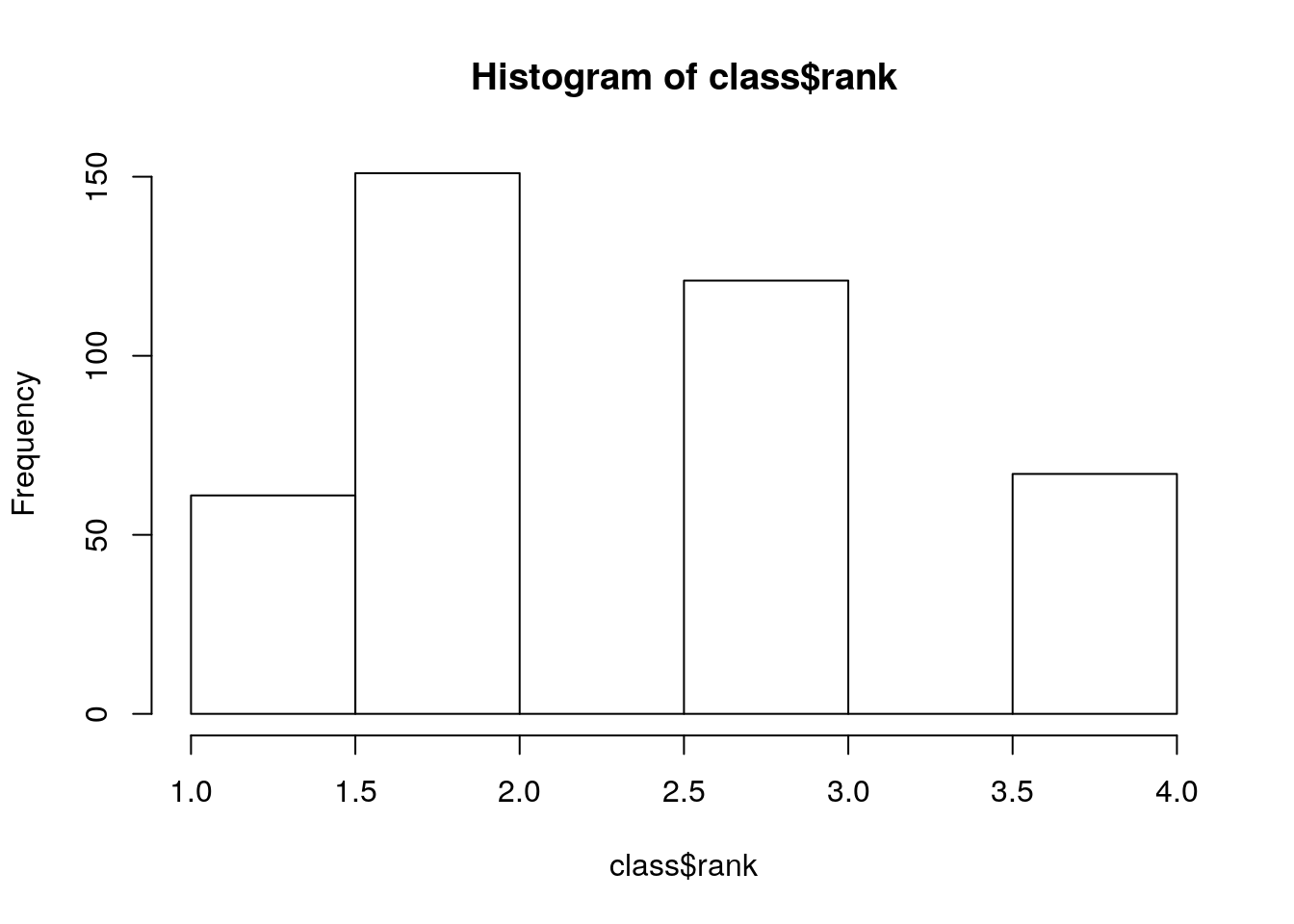
10.7.3 Running a logstic regression model
# Using the logit model: The code below estimates a logistic regression model using the glm (generalized linear model) function. First, we convert rank to a factor to indicate that rank should be treated as a categorical variable.
class$rank <- factor(class$rank)
mylogit <- glm(admit ~ gre + gpa + rank, data = class, family = "binomial")
# Check the result of our model
summary(mylogit)
##
## Call:
## glm(formula = admit ~ gre + gpa + rank, family = "binomial",
## data = class)
##
## Deviance Residuals:
## Min 1Q Median 3Q Max
## -1.6268 -0.8662 -0.6388 1.1490 2.0790
##
## Coefficients:
## Estimate Std. Error z value Pr(>|z|)
## (Intercept) -3.989979 1.139951 -3.500 0.000465 ***
## gre 0.002264 0.001094 2.070 0.038465 *
## gpa 0.804038 0.331819 2.423 0.015388 *
## rank2 -0.675443 0.316490 -2.134 0.032829 *
## rank3 -1.340204 0.345306 -3.881 0.000104 ***
## rank4 -1.551464 0.417832 -3.713 0.000205 ***
## ---
## Signif. codes: 0 '***' 0.001 '**' 0.01 '*' 0.05 '.' 0.1 ' ' 1
##
## (Dispersion parameter for binomial family taken to be 1)
##
## Null deviance: 499.98 on 399 degrees of freedom
## Residual deviance: 458.52 on 394 degrees of freedom
## AIC: 470.52
##
## Number of Fisher Scoring iterations: 4In the output above, the first thing we see is the call, this is R reminding us what the model we ran was, what options we specified, etc.
Next we see the deviance residuals, which are a measure of model fit. This part of output shows the distribution of the deviance residuals for individual cases used in the model. Below we discuss how to use summaries of the deviance statistic to assess model fit.
The next part of the output shows the coefficients, their standard errors, the z-statistic (sometimes called a Wald z-statistic), and the associated p-values. Both gre and gpa are statistically significant, as are the three terms for rank. The logistic regression coefficients give the change in the log odds of the outcome for a one unit increase in the predictor variable.
How to do the interpretation?
For every one unit change in gre, the log odds of admission (versus non-admission) increases by 0.002.
For a one unit increase in gpa, the log odds of being admitted to graduate school increases by 0.804.
The indicator variables for rank have a slightly different interpretation. For example, having attended an undergraduate institution with rank of 2, versus an institution with a rank of 1, changes the log odds of admission by -0.675.
Below the table of coefficients are fit indices, including the null and deviance residuals and the AIC. Later we show an example of how you can use these values to help assess model fit.
Why the coefficient value of rank (B) are different with the SPSS outputs? - In R, the glm automatically made the Rank 1 as the references group. However, in our SPSS example, we set the rank 4 as the reference group.
We can test for an overall effect of rank using the wald.test function of the aod library. The order in which the coefficients are given in the table of coefficients is the same as the order of the terms in the model. This is important because the wald.test function refers to the coefficients by their order in the model. We use the wald.test function. b supplies the coefficients, while Sigma supplies the variance covariance matrix of the error terms, finally Terms tells R which terms in the model are to be tested, in this case, terms 4, 5, and 6, are the three terms for the levels of rank.
##
## Attaching package: 'aod'
## The following object is masked from 'package:survival':
##
## rats## Wald test:
## ----------
##
## Chi-squared test:
## X2 = 20.9, df = 3, P(> X2) = 0.00011The chi-squared test statistic of 20.9, with three degrees of freedom is associated with a p-value of 0.00011 indicating that the overall effect of rank is statistically significant.
We can also test additional hypotheses about the differences in the coefficients for the different levels of rank. Below we test that the coefficient for rank=2 is equal to the coefficient for rank=3. The first line of code below creates a vector l that defines the test we want to perform. In this case, we want to test the difference (subtraction) of the terms for rank=2 and rank=3 (i.e., the 4th and 5th terms in the model). To contrast these two terms, we multiply one of them by 1, and the other by -1. The other terms in the model are not involved in the test, so they are multiplied by 0. The second line of code below uses L=l to tell R that we wish to base the test on the vector l (rather than using the Terms option as we did above).
# Prepare the comparison code
l <- cbind(0, 0, 0, 1, -1, 0)
# Run wald test to see whether Rank 2 is equal to Rank 3.
wald.test(b = coef(mylogit), Sigma = vcov(mylogit), L = l)
## Wald test:
## ----------
##
## Chi-squared test:
## X2 = 5.5, df = 1, P(> X2) = 0.019The chi-squared test statistic of 5.5 with 1 degree of freedom is associated with a p-value of 0.019, indicating that the difference between the coefficient for rank=2 and the coefficient for rank=3 is statistically significant.
You can also exponentiate the coefficients and interpret them as odds-ratios. R will do this computation for you. To get the exponentiated coefficients, you tell R that you want to exponentiate (exp), and that the object you want to exponentiate is called coefficients and it is part of mylogit (coef(mylogit)). We can use the same logic to get odds ratios and their confidence intervals, by exponentiating the confidence intervals from before. To put it all in one table, we use cbind to bind the coefficients and confidence intervals column-wise.
## (Intercept)         gre         gpa       rank2       rank3       rank4
##   0.0185001   1.0022670   2.2345451   0.5089309   0.2617923   0.2119375
## Waiting for profiling to be done...## OR 2.5 % 97.5 %
## (Intercept) 0.0185001 0.001889165 0.1665354
## gre 1.0022670 1.000137602 1.0044457
## gpa 2.2345451 1.173858341 4.3238354
## rank2 0.5089309 0.272289673 0.9448343
## rank3 0.2617923 0.131641715 0.5115181
## rank4 0.2119375 0.090715546 0.4706961Now we can say that for a one unit increase in gpa, the odds of being admitted to graduate school (versus not being admitted) increase by a factor of 2.23.
For more information on interpreting odds ratios see our FAQ page: How do I interpret odds ratios in logistic regression? Link:
Note that while R produces it, the odds ratio for the intercept is not generally interpreted.
You can also use predicted probabilities to help you understand the model. Predicted probabilities can be computed for both categorical and continuous predictor variables. In order to create predicted probabilities we first need to create a new data frame with the values we want the independent variables to take on to create our predictions
We will start by calculating the predicted probability of admission at each value of rank, holding gre and gpa at their means.
# First we create and view the data frame.
newdata1 <- with(class, data.frame(gre = mean(gre), gpa = mean(gpa), rank = factor(1:4)))

## view data frame
newdata1
## gre gpa rank
## 1 587.7 3.3899 1
## 2 587.7 3.3899 2
## 3 587.7 3.3899 3
## 4 587.7 3.3899 4These objects must have the same names as the variables in your logistic regression above (e.g. in this example the mean for gre must be named gre). Now that we have the data frame we want to use to calculate the predicted probabilities, we can tell R to create the predicted probabilities. The first line of code below is quite compact, we will break it apart to discuss what various components do. The newdata1$rankP tells R that we want to create a new variable in the dataset (data frame) newdata1 called rankP, the rest of the command tells R that the values of rankP should be predictions made using the predict( ) function. The options within the parentheses tell R that the predictions should be based on the analysis mylogit with values of the predictor variables coming from newdata1 and that the type of prediction is a predicted probability (type=“response”). The second line of the code lists the values in the data frame newdata1. Although not particularly pretty, this is a table of predicted probabilities.
# Add a predicted Rank column
newdata1$rankP <- predict(mylogit, newdata = newdata1, type = "response")
newdata1
## gre gpa rank rankP
## 1 587.7 3.3899 1 0.5166016
## 2 587.7 3.3899 2 0.3522846
## 3 587.7 3.3899 3 0.2186120
## 4 587.7 3.3899 4 0.1846684In the above output we see that the predicted probability of being accepted into a graduate program is 0.52 for students from the highest prestige undergraduate institutions (rank=1), and 0.18 for students from the lowest ranked institutions (rank=4), holding gre and gpa at their means.
Now, we are going to do something that do not exist in our SPSS section
# We can do something very similar to create a table of predicted probabilities varying the value of gre and rank.
# We are going to plot these, so we will create 100 values of gre between 200 and 800, at each value of rank (i.e., 1, 2, 3, and 4).
newdata2 <- with(class, data.frame(gre = rep(seq(from = 200, to = 800, length.out = 100), 4), gpa = mean(gpa), rank = factor(rep(1:4, each = 100))))
head(newdata2,10)
## gre gpa rank
## 1 200.0000 3.3899 1
## 2 206.0606 3.3899 1
## 3 212.1212 3.3899 1
## 4 218.1818 3.3899 1
## 5 224.2424 3.3899 1
## 6 230.3030 3.3899 1
## 7 236.3636 3.3899 1
## 8 242.4242 3.3899 1
## 9 248.4848 3.3899 1
## 10 254.5455 3.3899 1The code to generate the predicted probabilities (the first line below) is the same as before, except we are also going to ask for standard errors so we can plot a confidence interval. We get the estimates on the link scale and back transform both the predicted values and confidence limits into probabilities.
newdata3 <- cbind(newdata2, predict(mylogit, newdata = newdata2, type = "link",
    se = TRUE))
newdata3 <- within(newdata3, {
    PredictedProb <- plogis(fit)
    LL <- plogis(fit - (1.96 * se.fit))
    UL <- plogis(fit + (1.96 * se.fit))
})

## view first few rows of final dataset
head(newdata3)
## gre gpa rank fit se.fit residual.scale UL LL
## 1 200.0000 3.3899 1 -0.8114870 0.5147714 1 0.5492064 0.1393812
## 2 206.0606 3.3899 1 -0.7977632 0.5090986 1 0.5498513 0.1423880
## 3 212.1212 3.3899 1 -0.7840394 0.5034491 1 0.5505074 0.1454429
## 4 218.1818 3.3899 1 -0.7703156 0.4978239 1 0.5511750 0.1485460
## 5 224.2424 3.3899 1 -0.7565918 0.4922237 1 0.5518545 0.1516973
## 6 230.3030 3.3899 1 -0.7428680 0.4866494 1 0.5525464 0.1548967
## PredictedProb
## 1 0.3075737
## 2 0.3105042
## 3 0.3134500
## 4 0.3164108
## 5 0.3193867
## 6 0.3223773It can also be helpful to use graphs of predicted probabilities to understand and/or present the model. We will use the ggplot2 package for graphing.
# Load the ggplot2 for the plot
library(ggplot2)
# we make a plot with the predicted probabilities, and 95% confidence intervals.
ggplot(newdata3, aes(x = gre, y = PredictedProb)) + geom_ribbon(aes(ymin = LL,
    ymax = UL, fill = rank), alpha = 0.2) + geom_line(aes(colour = rank),
    size = 1)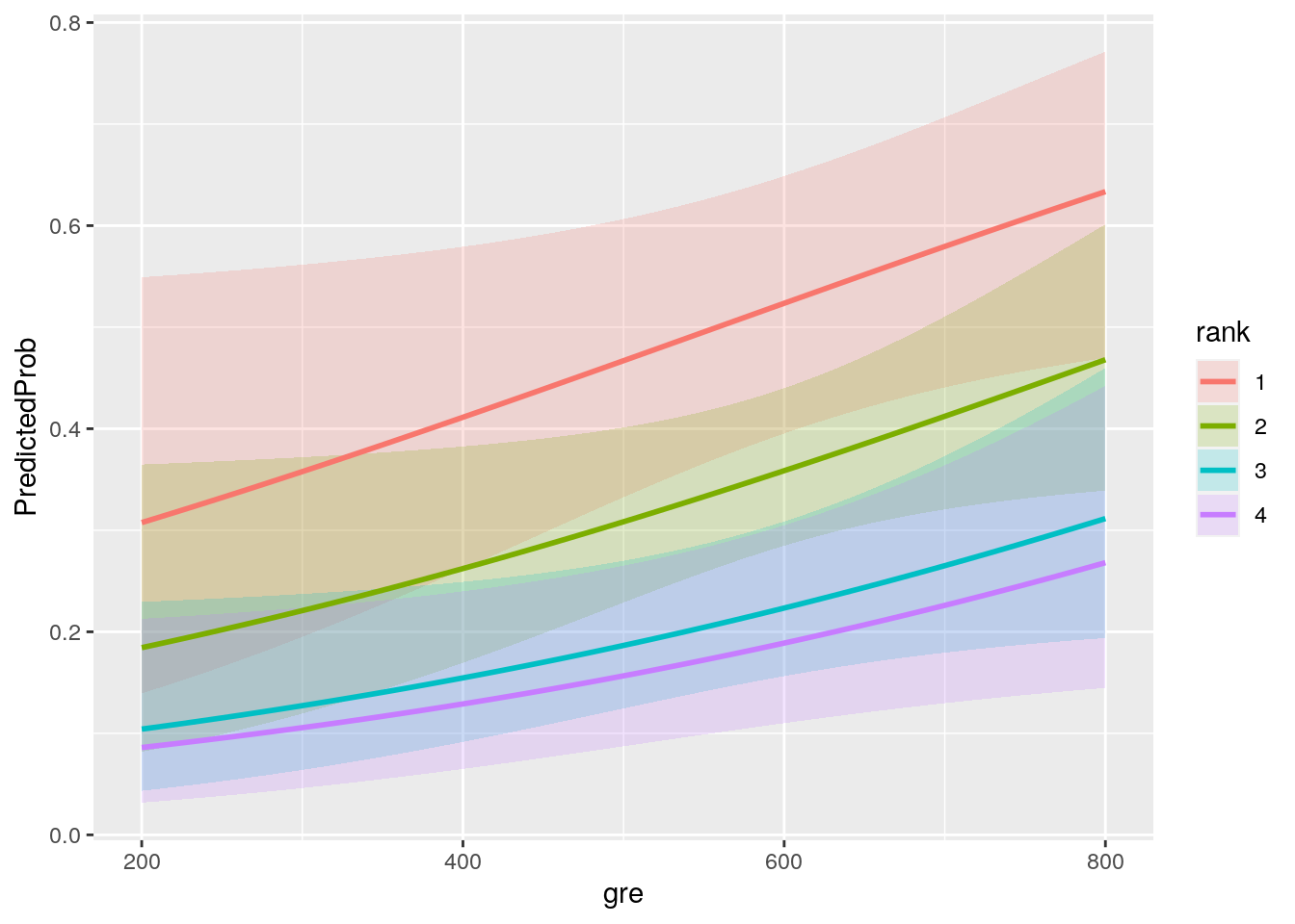
We may also wish to see measures of how well our model fits. This can be particularly useful when comparing competing models. The output produced by summary(mylogit) included indices of fit (shown below the coefficients), including the null and deviance residuals and the AIC. One measure of model fit is the significance of the overall model. This test asks whether the model with predictors fits significantly better than a model with just an intercept (i.e., a null model). The test statistic is the difference between the residual deviance for the model with predictors and the null model. The test statistic is distributed chi-squared with degrees of freedom equal to the differences in degrees of freedom between the current and the null model (i.e., the number of predictor variables in the model). To find the difference in deviance for the two models (i.e., the test statistic) we can use the command:
# The test statistic is the difference between the residual deviance for the model with predictors and the null model.
with(mylogit, null.deviance - deviance)
## [1] 41.45903# The degrees of freedom for the difference between the two models is equal to the number of predictor variables in the mode, and can be obtained using:
with(mylogit, df.null - df.residual)## [1] 5# Finally, the p-value can be obtained using:
with(mylogit, pchisq(null.deviance - deviance, df.null - df.residual, lower.tail = FALSE))## [1] 7.578189e-0810.8 Things to consider
Empty cells or small cells: You should check for empty or small cells by doing a crosstab between categorical predictors and the outcome variable. If a cell has very few cases (a small cell), the model may become unstable or it might not run at all.
Separation or quasi-separation (also called perfect prediction), a condition in which the outcome does not vary at some levels of the independent variables. See our page FAQ: What is complete or quasi-complete separation in logistic/probit regression and how do we deal with them? for information on models with perfect prediction. Link
Sample size: Both logit and probit models require more cases than OLS regression because they use maximum likelihood estimation techniques. It is sometimes possible to estimate models for binary outcomes in datasets with only a small number of cases using exact logistic regression. It is also important to keep in mind that when the outcome is rare, even if the overall dataset is large, it can be difficult to estimate a logit model.
Pseudo-R-squared: Many different measures of psuedo-R-squared exist. They all attempt to provide information similar to that provided by R-squared in OLS regression; however, none of them can be interpreted exactly as R-squared in OLS regression is interpreted. For a discussion of various pseudo-R-squareds see Long and Freese (2006) or our FAQ page What are pseudo R-squareds? Link
Diagnostics: The diagnostics for logistic regression are different from those for OLS regression. For a discussion of model diagnostics for logistic regression, see Hosmer and Lemeshow (2000, Chapter 5). Note that diagnostics done for logistic regression are similar to those done for probit regression.
10.9 Supplementary Learning Materials
Agresti, A. (1996). An Introduction to Categorical Data Analysis. Wiley & Sons, NY.
Burns, R. P. & Burns R. (2008). Business research methods & statistics using SPSS. SAGE Publications.
Field, A (2013). Discovering statistics using IBM SPSS statistics (4th ed.). Los Angeles, CA: Sage Publications