Chapter 13 Probit Analysis
13.1 Introduction to Probit Analysis
The probit function is the inverse of the cumulative distribution function of the standard normal distribution(i.e., N(0,1)), which is denoted as φ(z), so the probit is denoted as φ-1(p). φ(z) = p ↔︎ φ-1(p) = z (φ= phi)
Probit(p) = φ-1(p). Therefore, φ(probit(p)) = p and probit(φ(z)) = z.
Probitanalysis is used to model dichotomous or binary dependent variables.
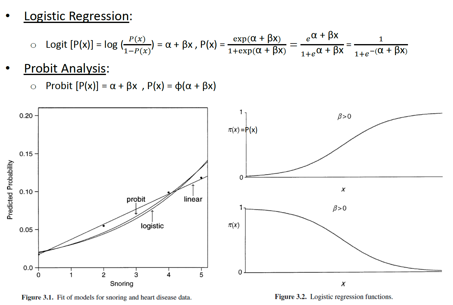
Logistic Regression vs. Probit Analysis
The fitted values, shown in above Figure 3.1, are similar to those for the linear probability and logistic regression models.
Probit and logit models are reasonable choices when the changes in the cumulative probabilities are gradual. In practice, probit and logistic regression models provide similar fits.
If a logistic regression model fits well, then so does the probit model, and conversely.
In general, probit analysis is appropriate for designed experiments, whereas logistic regression is more appropriate for observational studies.
13.2 R-Lab: Running Probit Analysis in R
13.2.1 Understanding the Data
R Example: Data Explanations (probit (=binary).sav)
A researcher is interested in how variables, such as GRE (Graduate Record Exam scores), GPA (grade point average) and prestige of the undergraduate institution, effect admission into graduate school. The response variable, admit/don’t admit, is a binary variable (binary.sav).
This dataset has a binary response (outcome, dependent) variable called admit, which is equal to 1 if the individual was admitted to graduate school, and 0 otherwise.
We will use recoded binary response variable called admit_re for this study. which is equal to 0 if the individual was admitted to graduate school, and 1 otherwise.
There are three predictor variables: GRE, GPA, and rank. We will treat the variables GRE and GPA as continuous. The variable rank takes on the values 1 through 4. Institutions with a rank of 1 have the highest prestige, while those with a rank of 4 have the lowest.
13.2.2 Descriptive data analysis
# Import the dataset into R
library(haven)
probit_binary_ <- read_sav("probit (=binary).sav")
# Prepare a copy for analysis
prob_data <- probit_binary_
# Take a glance of the data
summary(prob_data)
## admit admit_re gre gpa
## Min. :0.0000 Min. :0.0000 Min. :220.0 Min. :2.260
## 1st Qu.:0.0000 1st Qu.:0.0000 1st Qu.:520.0 1st Qu.:3.130
## Median :0.0000 Median :1.0000 Median :580.0 Median :3.395
## Mean :0.3175 Mean :0.6825 Mean :587.7 Mean :3.390
## 3rd Qu.:1.0000 3rd Qu.:1.0000 3rd Qu.:660.0 3rd Qu.:3.670
## Max. :1.0000 Max. :1.0000 Max. :800.0 Max. :4.000
## rank
## Min. :1.000
## 1st Qu.:2.000
## Median :2.000
## Mean :2.485
## 3rd Qu.:3.000
## Max. :4.000## tibble [400 × 5] (S3: tbl_df/tbl/data.frame)
## $ admit : dbl+lbl [1:400] 0, 1, 1, 1, 0, 1, 1, 0, 1, 0, 0, 0, 1, 0, 1, 0, 0, 0, ...
## ..@ format.spss : chr "F4.0"
## ..@ display_width: int 9
## ..@ labels : Named num [1:2] 0 1
## .. ..- attr(*, "names")= chr [1:2] "No=not admit" "Yes=admit"
## $ admit_re: dbl+lbl [1:400] 1, 0, 0, 0, 1, 0, 0, 1, 0, 1, 1, 1, 0, 1, 0, 1, 1, 1, ...
## ..@ format.spss : chr "F4.0"
## ..@ display_width: int 9
## ..@ labels : Named num [1:2] 0 1
## .. ..- attr(*, "names")= chr [1:2] "Yes=admit" "No=not admit"
## $ gre : num [1:400] 380 660 800 640 520 760 560 400 540 700 ...
## ..- attr(*, "format.spss")= chr "F3.0"
## ..- attr(*, "display_width")= int 9
## $ gpa : num [1:400] 3.61 3.67 4 3.19 2.93 ...
## ..- attr(*, "format.spss")= chr "F4.2"
## ..- attr(*, "display_width")= int 9
## $ rank : dbl+lbl [1:400] 3, 3, 1, 4, 4, 2, 1, 2, 3, 2, 4, 1, 1, 2, 1, 3, 4, 3, ...
## ..@ format.spss : chr "F1.0"
## ..@ display_width: int 9
## ..@ labels : Named num [1:4] 1 2 3 4
## .. ..- attr(*, "names")= chr [1:4] "highest" "high" "low" "lowest"# Re-level the data
prob_data$rank <- factor(prob_data$rank,levels=c(1,2,3,4),labels=c("highest", "high", "low", "lowest"))
prob_data$admit_re <- factor(prob_data$admit_re,levels=c(0,1),labels=c("admitted","not-admitted"))
# Build a frequency table
xtabs(~rank + admit_re, data = prob_data)## admit_re
## rank admitted not-admitted
## highest 33 28
## high 54 97
## low 28 93
## lowest 12 5513.2.3 Run the Probit logistic Regression model using stats package
# In order to run the Probit logistic regression model, we need the glm function from the stats package
library(stats)
# Build the Probit logistic Regression model
prob_model <- glm(admit_re ~ gre + gpa + rank, family = binomial(link = "probit"),
    data = prob_data)
## model summary
summary(prob_model)
##
## Call:
## glm(formula = admit_re ~ gre + gpa + rank, family = binomial(link = "probit"),
## data = prob_data)
##
## Deviance Residuals:
## Min 1Q Median 3Q Max
## -2.1035 -1.1560 0.6389 0.8710 1.6163
##
## Coefficients:
## Estimate Std. Error z value Pr(>|z|)
## (Intercept) 2.386836 0.673946 3.542 0.000398 ***
## gre -0.001376 0.000650 -2.116 0.034329 *
## gpa -0.477730 0.197197 -2.423 0.015410 *
## rankhigh 0.415399 0.194977 2.131 0.033130 *
## ranklow 0.812138 0.208358 3.898 9.71e-05 ***
## ranklowest 0.935899 0.245272 3.816 0.000136 ***
## ---
## Signif. codes: 0 '***' 0.001 '**' 0.01 '*' 0.05 '.' 0.1 ' ' 1
##
## (Dispersion parameter for binomial family taken to be 1)
##
## Null deviance: 499.98 on 399 degrees of freedom
## Residual deviance: 458.41 on 394 degrees of freedom
## AIC: 470.41
##
## Number of Fisher Scoring iterations: 413.2.4 Compare the overall model fit
# Run a "only intercept" model
OIM <- glm(admit_re ~ 1,family = binomial(link = "probit"), data = prob_data)
summary(OIM)##
## Call:
## glm(formula = admit_re ~ 1, family = binomial(link = "probit"),
## data = prob_data)
##
## Deviance Residuals:
## Min 1Q Median 3Q Max
## -1.5148 -1.5148 0.8741 0.8741 0.8741
##
## Coefficients:
## Estimate Std. Error z value Pr(>|z|)
## (Intercept) 0.4747 0.0653 7.27 3.61e-13 ***
## ---
## Signif. codes: 0 '***' 0.001 '**' 0.01 '*' 0.05 '.' 0.1 ' ' 1
##
## (Dispersion parameter for binomial family taken to be 1)
##
## Null deviance: 499.98 on 399 degrees of freedom
## Residual deviance: 499.98 on 399 degrees of freedom
## AIC: 501.98
##
## Number of Fisher Scoring iterations: 4## Analysis of Deviance Table
##
## Model 1: admit_re ~ 1
## Model 2: admit_re ~ gre + gpa + rank
## Resid. Df Resid. Dev Df Deviance F Pr(>F)
## 1 399 499.98
## 2 394 458.41 5 41.563 8.3127 7.219e-08 ***
## ---
## Signif. codes: 0 '***' 0.001 '**' 0.01 '*' 0.05 '.' 0.1 ' ' 1Before proceeding to examine the individual coefficients, you want to look at an overall test of the null hypothesis that the location coefficients (βs) for all of the variables in the model are 0.
From the table, you see that the chi-square is 41.563 and p < .001. This means that you can reject the null hypothesis that the model without predictors is as good as the model with the predictors.
\(H_0\): The model is a good fitting to the null model
\(H_1\): The model is not a good fitting to the null model (i.e. the predictors have a significant effect)
13.2.5 Check the model fit information
## 1 2 3 4 5 6 7 8
## 0.8293613 0.7046477 0.2661311 0.8207949 0.8864147 0.6268783 0.5764696 0.7824784
## 9 10 11 12 13 14 15 16
## 0.7986055 0.4866859 0.6222300 0.5961079 0.2844973 0.6435312 0.3131301 0.8146865
## 17 18 19 20
## 0.6557750 0.9306664 0.4642531 0.4300943##
## Pearson's Chi-squared test
##
## data: prob_data$admit_re and predict(prob_model)
## X-squared = 390, df = 390, p-value = 0.4905From the observed and expected frequencies, you can compute the usual Pearson and Deviance goodness-of-fit measures. You can chose either A or B options to report the goodness-of-fit.
Both of the goodness-of-fit statistics should be used only for models that have reasonably large expected values in each cell. If you have a continuous independent variable or many categorical predictors or some predictors with many values, you may have many cells with small expected values.
If your model fits well (p > .05), the observed and expected cell counts are similar. In other words, the model fits the data well.
13.2.6 Measuring Strength of Association (Calculating the Pseudo R-Square)
# Load the DescTools package for calculate the R square
# library("DescTools")
# Calculate the R Square
# PseudoR2(prob_model, which = c("CoxSnell","Nagelkerke","McFadden"))There are several R2-like statistics that can be used to measure the strength of the association between the dependent variable and the predictor variables.
They are not as useful as the statistic in multiple regression, since their interpretation is not straightforward.
For this example, there is the relationship of 13.8% between independent variables and dependent variable based on Nagelkerke’s R2.
13.2.7 Parameter Estimates
##
## Call:
## glm(formula = admit_re ~ gre + gpa + rank, family = binomial(link = "probit"),
##     data = prob_data)
##
## Deviance Residuals:
##     Min       1Q   Median       3Q      Max
## -2.1035  -1.1560   0.6389   0.8710   1.6163
##
## Coefficients:
##              Estimate Std. Error z value Pr(>|z|)
## (Intercept)  2.386836   0.673946   3.542 0.000398 ***
## gre         -0.001376   0.000650  -2.116 0.034329 *
## gpa         -0.477730   0.197197  -2.423 0.015410 *
## rankhigh     0.415399   0.194977   2.131 0.033130 *
## ranklow      0.812138   0.208358   3.898 9.71e-05 ***
## ranklowest   0.935899   0.245272   3.816 0.000136 ***
## ---
## Signif. codes:  0 '***' 0.001 '**' 0.01 '*' 0.05 '.' 0.1 ' ' 1
##
## (Dispersion parameter for binomial family taken to be 1)
##
##     Null deviance: 499.98  on 399  degrees of freedom
## Residual deviance: 458.41  on 394  degrees of freedom
## AIC: 470.41
##
## Number of Fisher Scoring iterations: 4# We can use the coef() function to check the parameter estimates
(Prob_estimates <- coef(summary(prob_model)))## Estimate Std. Error z value Pr(>|z|)
## (Intercept) 2.386836491 0.6739460869 3.541584 3.977326e-04
## gre -0.001375591 0.0006500337 -2.116184 3.432919e-02
## gpa -0.477730110 0.1971968582 -2.422605 1.540967e-02
## rankhigh 0.415399408 0.1949766644 2.130508 3.312967e-02
## ranklow 0.812138084 0.2083576222 3.897808 9.706718e-05
## ranklowest 0.935899179 0.2452719184 3.815762 1.357635e-04Note: Please note the intercept estimate and the rank estimates are different between R and SPSS, that is because in R, it takes the different reference group. The default setting is use 1 as the reference group.
In the output above, the first thing we see is the call, this is R reminding us what the model we ran was, what options we specified, etc.
Next we see the deviance residuals, which are a measure of model fit. This part of output shows the distribution of the deviance residuals for individual cases used in the model. Below we discuss how to use summaries of the deviance statistic to asses model fit.
The next part of the output shows the coefficients, their standard errors, the z-statistic (sometimes called a Wald z-statistic), and the associated p-values. Both gre, gpa, and the three terms for rank are statistically significant. The probit regression coefficients give the change in the z-score or probit index for a one unit change in the predictor.
For a one unit increase in gre, the z-score decreases by 0.001.
For each one unit increase in gpa, the z-score decreases by 0.478.
The indicator variables for rank have a slightly different interpretation. For example, having attended an undergraduate institution of rank of 2, versus an institution with a rank of 1 (the reference group), increases the z-score by 0.415.
Below the table of coefficients are fit indices, including the null and deviance residuals and the AIC.
13.3 Supplementary Learning Materials
Agresti, A. (1996). An introduction to categorical data analysis. New York, NY: Wiley & Sons. Chapter 3. Generalized Linear Models.