Chapter 5 Multiple Regression
5.1 Introduction to Multiple Regression
Multiple regression is an extension of simple linear regression. It is used when we want to predict the value of a variable based on the value of two or more other variables. The variable we want to predict is called the dependent variable (or sometimes, the outcome, target or criterion variable).
5.2 Simple Regression using R
5.2.1 Load your data
# Load the haven package to use read_sav function
library(haven)
# Use read_sav function to import the data into R
regression_data <- read_sav("asgusam5(regression).sav")
# Take a preview of the data
head(regression_data,10)
## # A tibble: 10 x 58
## id gender month year language book home_computer home_desk
## <dbl> <dbl+l> <dbl+lb> <dbl+l> <dbl+lb> <dbl+l> <dbl+lbl> <dbl+lbl>
## 1 1 1 [GIR… 1 [JAN… 5 [200… 1 [ALWA… 4 [TWO… 1 [YES] 0 [NO]
## 2 2 0 [BOY] 9 [SEP… 4 [200… 1 [ALWA… 3 [ONE… 1 [YES] 1 [YES]
## 3 3 0 [BOY] 10 [OCT… 4 [200… 1 [ALWA… 4 [TWO… 1 [YES] 1 [YES]
## 4 4 1 [GIR… 8 [AUG… 4 [200… 1 [ALWA… 3 [ONE… 1 [YES] 1 [YES]
## 5 5 0 [BOY] 8 [AUG… 4 [200… 1 [ALWA… 5 [THR… 1 [YES] 1 [YES]
## 6 6 0 [BOY] 11 [NOV… 4 [200… 1 [ALWA… 3 [ONE… 1 [YES] 1 [YES]
## 7 7 1 [GIR… 1 [JAN… 4 [200… 1 [ALWA… 2 [ONE… 1 [YES] 1 [YES]
## 8 8 1 [GIR… 11 [NOV… 4 [200… 1 [ALWA… 3 [ONE… 1 [YES] 1 [YES]
## 9 9 0 [BOY] 8 [AUG… 4 [200… 1 [ALWA… 4 [TWO… 1 [YES] 1 [YES]
## 10 10 1 [GIR… 6 [JUN… 4 [200… 1 [ALWA… 2 [ONE… 0 [NO] 1 [YES]
## # … with 50 more variables: home_book <dbl+lbl>, home_room <dbl+lbl>,
## # home_internet <dbl+lbl>, computer_home <dbl+lbl>,
## # computer_school <dbl+lbl>, computer_some <dbl+lbl>,
## # parentsupport1 <dbl+lbl>, parentsupport2 <dbl+lbl>,
## # parentsupport3 <dbl+lbl>, parentsupport4 <dbl+lbl>, school1 <dbl+lbl>,
## # school2 <dbl+lbl>, school3 <dbl+lbl>, studentbullied1 <dbl+lbl>,
## # studentbullied2 <dbl+lbl>, studentbullied3 <dbl+lbl>,
## # studentbullied4 <dbl+lbl>, studentbullied5 <dbl+lbl>,
## # studentbullied6 <dbl+lbl>, learning1 <dbl+lbl>, learning2 <dbl+lbl>,
## # learning3 <dbl+lbl>, learning4 <dbl+lbl>, learning5 <dbl+lbl>,
## # learning6 <dbl+lbl>, learning7 <dbl+lbl>, engagement1 <dbl+lbl>,
## # engagement2 <dbl+lbl>, engagement3 <dbl+lbl>, engagement4 <dbl+lbl>,
## # engagement5 <dbl+lbl>, confidence1 <dbl+lbl>, confidence2 <dbl+lbl>,
## # confidence3 <dbl+lbl>, confidence4 <dbl+lbl>, confidence5 <dbl+lbl>,
## # confidence6 <dbl+lbl>, score1 <dbl>, score2 <dbl>, score3 <dbl>,
## # score4 <dbl>, score5 <dbl>, ParentSupport <dbl>, Home <dbl>, school <dbl>,
## # StudentBullied <dbl>, learning <dbl>, engagement <dbl>, confidence <dbl>,
## # ScienceScore <dbl>5.2.2 Scatterplot the data
# load the ggplot2 package to use the ggplot() function
library(ggplot2)
# Scatterplot the data by using ggplot() function between confidence and Science Score
ggplot(regression_data,aes(x=confidence,y=ScienceScore))+geom_point()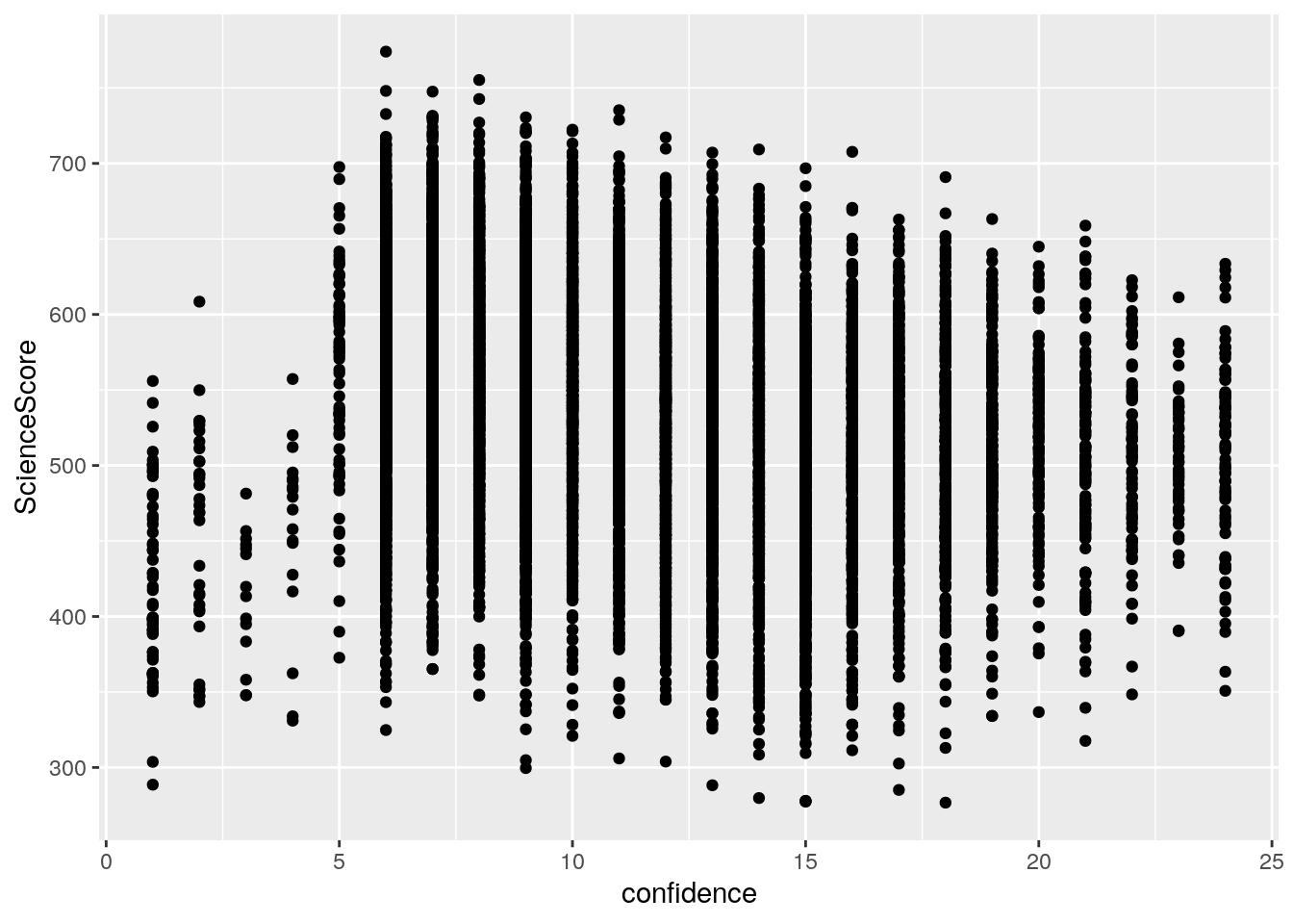
## Alternative approach: You can also use the sactter.smooth() function to run the scatterplot
scatter.smooth(x=regression_data$confidence,y=regression_data$ScienceScore,main="Confindence ~ ScienceScore")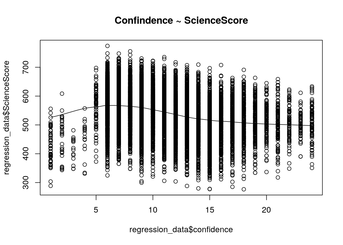
5.2.3 Check the correlation
From the scatterplot, it is hard to tell whether there is a positive or negative relationship between two variables.
# Check the correlation
cor(regression_data$confidence,regression_data$ScienceScore,use="pairwise.complete.obs",method="pearson")
## [1] -0.27727545.2.4 Run a simple regression model
Now that we have seen the linear relationship pictorially in the scatter plot and by computing the correlation, lets see the syntax for building the linear model.
# The function used for building linear models is lm(). The lm() function takes in two main arguments, namely: 1. Formula 2. Data. The data is typically a data.frame and the formula is a object of class formula. But the most common convention is to write out the formula directly in place of the argument as written below.
Simple_Reg <- lm(ScienceScore ~ confidence, data=regression_data)
# Check the Model we ran
summary(Simple_Reg)
##
## Call:
## lm(formula = ScienceScore ~ confidence, data = regression_data)
##
## Residuals:
## Min 1Q Median 3Q Max
## -299.890 -46.360 4.834 50.316 209.564
##
## Coefficients:
## Estimate Std. Error t value Pr(>|t|)
## (Intercept) 593.3307 1.6898 351.12 <2e-16 ***
## confidence -4.8103 0.1472 -32.69 <2e-16 ***
## ---
## Signif. codes: 0 '***' 0.001 '**' 0.01 '*' 0.05 '.' 0.1 ' ' 1
##
## Residual standard error: 71.32 on 12829 degrees of freedom
## (238 observations deleted due to missingness)
## Multiple R-squared: 0.07688, Adjusted R-squared: 0.07681
## F-statistic: 1068 on 1 and 12829 DF, p-value: < 2.2e-16Check your SPSS outputs, could you find all the corrsponding key values in your R outcome.
Check your class notes for the detailed interpretation
5.2.5 Centering Variable for better interpretation
# Load the package dplyr to use the mutate() function
library(dplyr)
# Get the mean for confidence variable
mean_confidence <- mean(na.omit(regression_data$confidence))
mean_confidence # The mean is equal to 10.66
## [1] 10.6563# Create a new variable: Centered_confidence
regression_data$Centered_confidence <- regression_data$confidence-10.66
# Rerun the simple regression model
Simple_Reg_centered <- lm(ScienceScore ~ Centered_confidence, data=regression_data)
# Check the Model we ran
summary(Simple_Reg_centered)##
## Call:
## lm(formula = ScienceScore ~ Centered_confidence, data = regression_data)
##
## Residuals:
## Min 1Q Median 3Q Max
## -299.890 -46.360 4.834 50.316 209.564
##
## Coefficients:
## Estimate Std. Error t value Pr(>|t|)
## (Intercept) 542.0532 0.6296 860.97 <2e-16 ***
## Centered_confidence -4.8103 0.1472 -32.69 <2e-16 ***
## ---
## Signif. codes: 0 '***' 0.001 '**' 0.01 '*' 0.05 '.' 0.1 ' ' 1
##
## Residual standard error: 71.32 on 12829 degrees of freedom
## (238 observations deleted due to missingness)
## Multiple R-squared: 0.07688, Adjusted R-squared: 0.07681
## F-statistic: 1068 on 1 and 12829 DF, p-value: < 2.2e-16Check your class notes for the detailed interpretation
5.3 Multiple Regression
5.3.1 Variable Selection Methods
Purpose: The purpose of variable selection is to select the minimum number of variables necessary to account for almost as much as the variance as is accounted for by the total set.
Weakness: The solution is not stable. When a different subset of predictors is identified, the order of variables enterend will vary.
Types of variable selection:
Enter: All independent variables are entered into the equation in one step, also called “forced entry”.
Forward selection: From a pool of potential predictors, the forward method adds one predictor at a time to a regression model until adding any additional variables dodes not explain any significant variation in the criterion variable. The main limitation with the forward method is that once a variable is added to the model it cannot be dropped.
Backward Elimination: The backward method begins all of the variables entered into a regression model and the goal is to drop one variable at a time until dropping a variable significantly reduces the R square statistic. The backward method has the same limitation as the forward method - that is once a variable is dropped is no longer considered for inclusion in the subset of best predictors.
Stepwise: The stepwise method begins the same as the forward method. But when a variable is added to the model all of the previously added variables are re-evaluated. So that a variable entered at step one may be dropped at step four but then added late at step six. Stepwise continues adding and deleting variables until the addition of new variables do not increase R square statistic significantly. Stepwise is therefore a combination of the forward and backward methods.
Note: Since the class do not provide examples on this topic, the R section here accordingly don’t provide you any examples. For further knowledge, you can visit here.
5.4 Assessing the regression model
# Prepare the dataset we need
multiple_regdata <- regression_data[ ,c("ScienceScore","Centered_confidence","gender","book")]
5.4.1 Run the Multiple Regression model
# We can still using the lm() function to run the multiple regression model (the formula will be different)
multiple_Reg <- lm(ScienceScore ~ Centered_confidence + gender + book, data=multiple_regdata)
# Check the Model we ran
summary(multiple_Reg)
##
## Call:
## lm(formula = ScienceScore ~ Centered_confidence + gender + book,
## data = multiple_regdata)
##
## Residuals:
## Min 1Q Median 3Q Max
## -304.599 -42.444 5.808 46.861 227.855
##
## Coefficients:
## Estimate Std. Error t value Pr(>|t|)
## (Intercept) 488.2018 1.6543 295.105 < 2e-16 ***
## Centered_confidence -3.9359 0.1402 -28.064 < 2e-16 ***
## gender -8.8173 1.1886 -7.418 1.26e-13 ***
## book 20.5240 0.5081 40.397 < 2e-16 ***
## ---
## Signif. codes: 0 '***' 0.001 '**' 0.01 '*' 0.05 '.' 0.1 ' ' 1
##
## Residual standard error: 66.8 on 12694 degrees of freedom
## (371 observations deleted due to missingness)
## Multiple R-squared: 0.184, Adjusted R-squared: 0.1838
## F-statistic: 954.3 on 3 and 12694 DF, p-value: < 2.2e-165.5 Assumptions
5.5.1 Check the correlation matrix & the P-value matrix
# Load the Hmisc package to run the correlation matrix
library(Hmisc)
# Since the rcorr() function do not allow missing values, we need clean the data first
cleaned_multiple_regdata <- na.omit(sapply(multiple_regdata,haven::zap_labels))
# Use the rcorr() function to obtain the correlation matrix and p-value matrix
rcorr(cleaned_multiple_regdata,type="pearson")
## ScienceScore Centered_confidence gender book
## ScienceScore 1.00 -0.28 -0.06 0.36
## Centered_confidence -0.28 1.00 0.05 -0.14
## gender -0.06 0.05 1.00 0.04
## book 0.36 -0.14 0.04 1.00
##
## n= 12698
##
##
## P
## ScienceScore Centered_confidence gender book
## ScienceScore 0 0 0
## Centered_confidence 0 0 0
## gender 0 0 0
## book 0 0 0Check that correlation between the dependent variable and independent variables are significant and the independent variables are not highly correlated each other.
5.5.2 Check the independent errors
Durbin-Waston Statistic is used to test for the presense of serial correlation among the residuals.
The value of the Durbin-Watson statistic ranges from 0 to 4. As a general rule of thumb, the residuals are uncorrelated is the Durbin-Watson statistic is approximately 2. A value close to 0 indicates strong positive correlation, while a value of 4 indicates strong negative correlation.
# Load the lmtest package to run the Durbin-Watson test
library(lmtest)
# Run the Durbin-Watson test by use dwtest() function (Note that the formula is the same as the multiple regression formula we just ran)
dwtest(ScienceScore ~ Centered_confidence + gender + book, data=multiple_regdata)
##
## Durbin-Watson test
##
## data: ScienceScore ~ Centered_confidence + gender + book
## DW = 1.4255, p-value < 2.2e-16
## alternative hypothesis: true autocorrelation is greater than 0From the output we can see, the value of Durbin-Waston is 1.426, close to 2, indicating no serial correlation.
5.5.3 Check the outliers by using Mahalanobis Distance
# Use the mahalanobis() function to calculate the mahalanobis distance
?mahalanobis() #check the function help page to see how to use the arguments
# According to the help page, we need mean vector and a corvariance matrix to calculate the mahalanobis distance.
colmean <- colMeans(cleaned_multiple_regdata)
Sx <- cov(cleaned_multiple_regdata)
# Calculate the mahalanobis distance
D2 <- mahalanobis(cleaned_multiple_regdata, colmean, Sx,inverted=FALSE)
mean(D2)
## [1] 3.999685The Mean distance is 3.99, which is less than 25, which means we are safe.
5.5.4 Check the outliers by using Cook’s Distance
# We can use cooks.distance() function to calculate the cook's distance. It is also in the stats package.
CD <- cooks.distance(multiple_Reg)
mean(CD)
## [1] 8.363979e-05## [1] 0.003131912The mean cook’s distance is really close to 0. And the max cook’s D is 0.003.
5.5.5 Check the other assumptions
# We can use plot("model name") to obtain four different plots to check the assumption of multiple regression.
plot(multiple_Reg)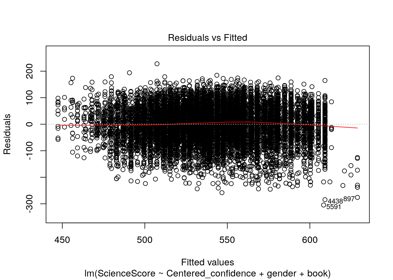
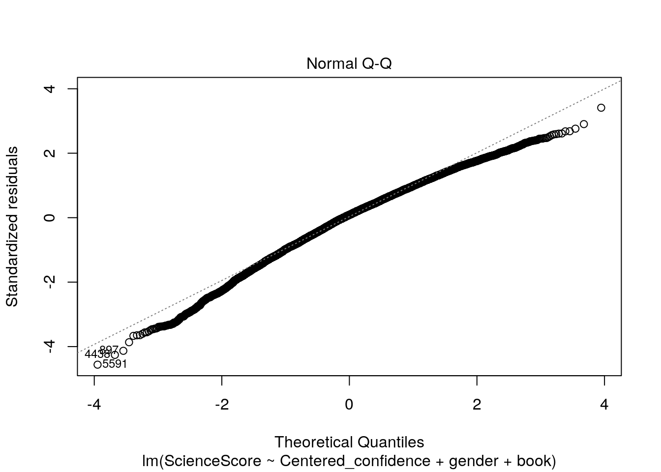
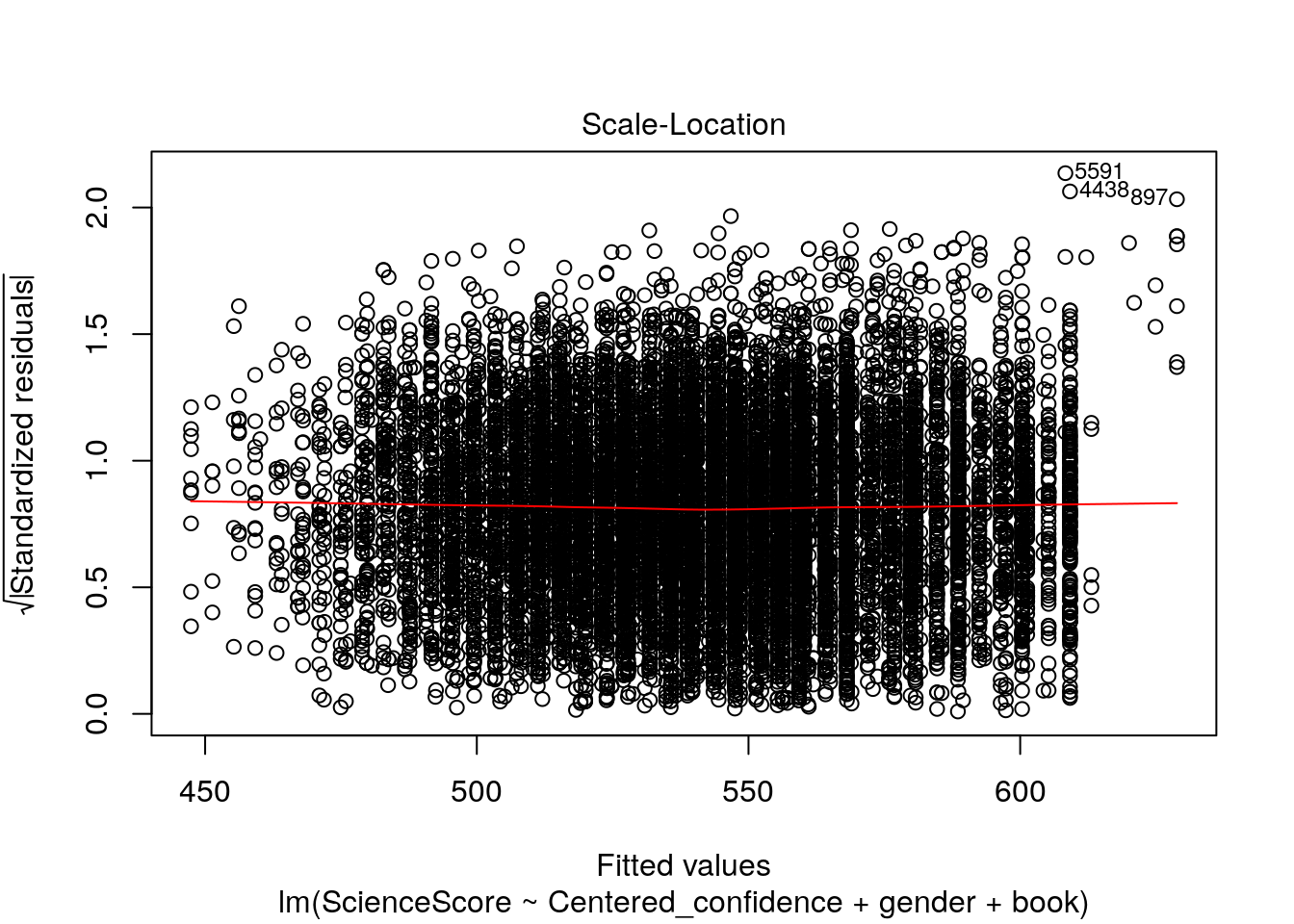
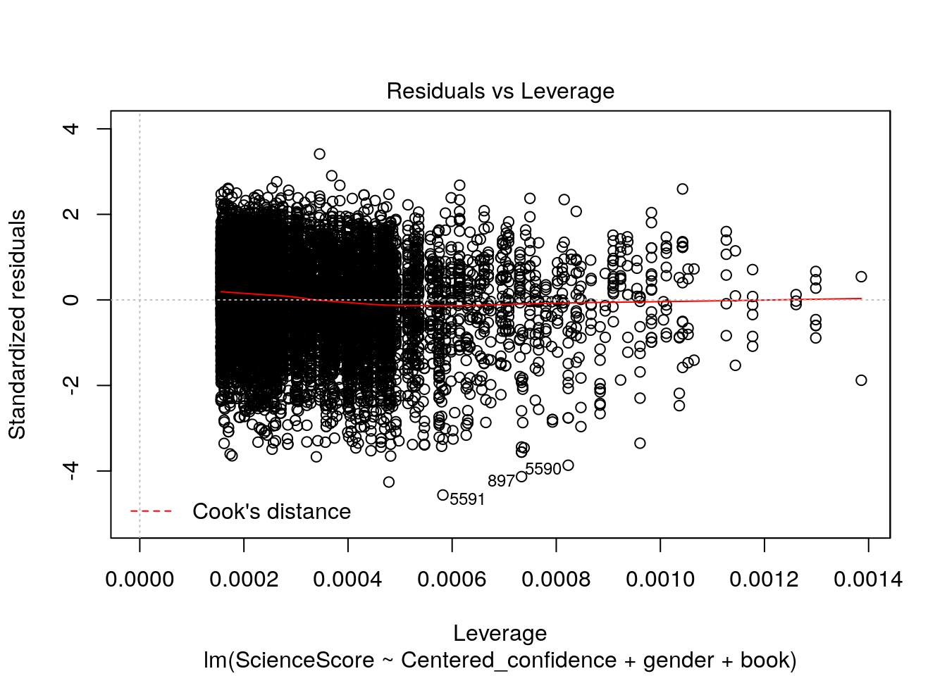
Now let’s check out these four wonderful plots above.
The diagnostic plots show residuals in four different ways:
1.Residuals vs Fitted. Used to check the linear relationship assumptions. A horizontal line, without distinct patterns is an indication for a linear relationship, what is good.
2.Normal Q-Q. Used to examine whether the residuals are normally distributed. It’s good if residuals points follow the straight dashed line.
3.Scale-Location (or Spread-Location). Used to check the homogeneity of variance of the residuals (homoscedasticity). Horizontal line with equally spread points is a good indication of homoscedasticity.
4.Residuals vs Leverage. Used to identify influential cases, that is extreme values that might influence the regression results when included or excluded from the analysis.
# Wait, comparing to our SPSS section, we don't have the histogram yet. No worry, here we go.
hist(multiple_Reg$residuals)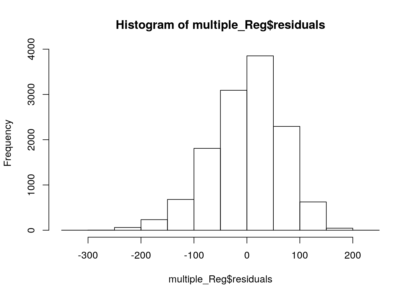
# Now we need standardize() function in robustHD package to standaarize our residuals.
library(robustHD)
hist(standardize(multiple_Reg$residuals))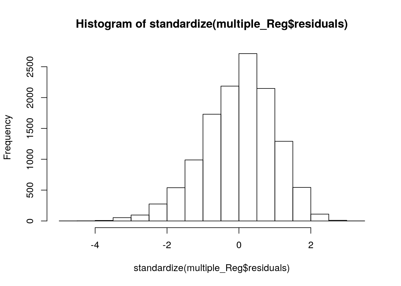
Now, the variables on X-axis (Standardized Residual) and Y-aixs (Frequency) are exactly the same with our SPSS version. However, the scale looks different. Could you figure out how to set these scales by yourself?
# Also, we need to check the Variance Inflation Factor (VIF) value to check the multicollinearity of the data
library(fmsb)
VIF(multiple_Reg)
## [1] 1.225532This indicates the VIF of the whole mode, the value is 1.23. If VIF is more than 10, multicolinearity is strongly suggested.
Interpretation
Since the interpretations are pretty much the same, please take the references on your class notes.