Chapter 12 Ordinal Logistic Regression
12.1 Introduction to Ordinal Logistic Regression
Ordinal Logistic Regression is used when there are three or more categories with a natural ordering to the levels, but the ranking of the levels do not necessarily mean the intervals between them are equal.
Examples of ordinal responses could be:
The effectiveness rating of a college course on a scale of 1-5
Levels of flavors for hot wings
Medical condition (e.g., good, stable, serious, critical)
Diseases can be graded on scales from least severe to most severe
Survey respondents choose answers on scales from strongly agree to strongly disagree
Students are graded on scales from A to F
12.2 Cumulative Probability
When response categories are ordered, the logits can utilize the ordering. You can modify the binary logistic regression model to incorporate the ordinal nature of a dependent variable by defining the probabilities differently.
Instead of considering the probability of an individual event, you consider the probabilities of that event and all events that are ordered before it.
A cumulative probability for \(Y\) is the probability that \(Y\) falls at or below a particular point. For outcome category \(j\), the cumulative probability is: \[P(Y \leq j)=\pi_{1}+\ldots+\pi_{j}, \mathrm{j}=1, \ldots, \mathrm{J}\] where \(𝜋_𝑗\) is the probability to chose category \(j\)
12.3 Link Function
The link function is the function of the probabilities that results in a linear model in the parameters.
Five different link functions are available in the Ordinal Regression procedure in SPSS: logit, complementary log-log, negative log-log, probit, and Cauchit (inverse Cauchy)
The symbol \(ϒ\) (gamma) represents the probability that the event occurs. Remember that in ordinal regression, the probability of an event is redefined in terms of cumulative probabilities.
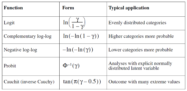
Table 1. The link function
Probit and logit models are reasonable choices when the changes in the cumulative probabilities are gradual. If there are abrupt changes, other link functions should be used.
The complementary log-log link may be a good model when the cumulative probabilities increase from 0 fairly slowly and then rapidly approach 1.
If the opposite is true, namely that the cumulative probability for lower scores is high and the approach to 1 is slow, the negative log-log link may describe the data.
12.4 Prepare the Data
Data Information (Agresti (1996), Table 6.9, p. 186)
Data set (impairment.sav) comes from a study of mental health for a random sample of adult residents of Alachua County, Florida. Mental impairment is ordinal, with categories (1 = well, 2 = mild symptom formation, 3 = moderate symptom formation, 4 = impaired).
The study related Y = mental impairment to two explanatory variables. The life events is a composite measure of the number and severity of important life events such as birth of child, new job, divorce, or death in family that occurred to the subject within the past three years. In this sample it has a mean of 4.3 and standard deviation of 2.7. Socioeconomic status (SES) is measured here as binary (0 = low & 1 = high).
## # A tibble: 6 x 4
##   subject  Impairment        ses lifeevents
##     <dbl>   <dbl+lbl>  <dbl+lbl>      <dbl>
## 1       1 1 [1= Well] 1 [1=high]          1
## 2       2 1 [1= Well] 1 [1=high]          9
## 3       3 1 [1= Well] 1 [1=high]          4
## 4       4 1 [1= Well] 1 [1=high]          3
## 5       5 1 [1= Well] 0 [0=low]           2
## 6       6 1 [1= Well] 1 [1=high]          0
# Prepare a copy for exercise
OLR_data <- impairment
# Ordering the dependent variable
OLR_data$Impairment <- factor(OLR_data$Impairment,levels=c(1,2,3,4),labels=c("well","mild","moderate","impaired"))
# Ordering the independent variable
OLR_data$ses <- factor(OLR_data$ses,levels=c(0,1),labels=c("low","high"))12.5 Descriptive Analysis
##     subject         Impairment   ses       lifeevents
##  Min.   : 1.00   well    :12   low :18   Min.   :0.000
##  1st Qu.:10.75   mild    :12   high:22   1st Qu.:2.000
##  Median :20.50   moderate: 7             Median :4.000
##  Mean   :20.50   impaired: 9             Mean   :4.275
##  3rd Qu.:30.25                           3rd Qu.:6.250
## Max. :40.00 Max. :9.000##
## low high
## well 4 8
## mild 4 8
## moderate 5 2
## impaired 5 4##
## 0 1 2 3 4 5 6 7 8 9
## well 1 3 2 3 1 0 0 1 0 1
## mild 0 2 1 3 0 3 1 0 1 1
## moderate 1 0 0 2 2 0 1 0 0 1
## impaired 0 0 1 0 2 1 0 1 3 112.6 Run the ordinal logistic Regression model using MASS package
# In order to run the ordinal logistic regression model, we need the polr function from the MASS package
library(MASS)
# Build ordinal logistic regression model
OLRmodel <- polr(Impairment ~ ses + lifeevents , data = OLR_data, Hess = TRUE)
summary(OLRmodel)
## Call:
## polr(formula = Impairment ~ ses + lifeevents, data = OLR_data,
## Hess = TRUE)
##
## Coefficients:
## Value Std. Error t value
## seshigh -1.1112 0.6109 -1.819
## lifeevents 0.3189 0.1210 2.635
##
## Intercepts:
## Value Std. Error t value
## well|mild -0.2819 0.6423 -0.4389
## mild|moderate 1.2128 0.6607 1.8357
## moderate|impaired 2.2094 0.7210 3.0644
##
## Residual Deviance: 99.0979
## AIC: 109.0979##
## Re-fitting to get Hessian## Call:
## polr(formula = Impairment ~ 1, data = OLR_data)
##
## No coefficients
##
## Intercepts:
## Value Std. Error t value
## well|mild -0.8473 0.3450 -2.4557
## mild|moderate 0.4055 0.3227 1.2562
## moderate|impaired 1.2368 0.3786 3.2663
##
## Residual Deviance: 109.0421
## AIC: 115.042112.7 Check the Overall Model Fit
## Likelihood ratio tests of ordinal regression models
##
## Response: Impairment
##              Model Resid. df Resid. Dev   Test    Df LR stat.     Pr(Chi)
## 1                1        37   109.0421
## 2 ses + lifeevents        35    99.0979 1 vs 2     2 9.944156 0.006928734
Before proceeding to examine the individual coefficients, you want to look at an overall test of the null hypothesis that the location coefficients for all of the variables in the model are 0.
You can base this on the change in log-likelihood when the variables are added to a model that contains only the intercept. The change in likelihood function has a chi-square distribution even when there are cells with small observed and predicted counts.
From the table, you see that the chi-square is 9.944 and p = .007. This means that you can reject the null hypothesis that the model without predictors is as good as the model with the predictors.
12.8 Check the model fit information
##          well      mild   moderate   impaired
## 1  0.62491585 0.2564222 0.07131474 0.04734725
## 2  0.11502358 0.2518325 0.24398557 0.38915837
## 3  0.39028430 0.3502175 0.14495563 0.11454256
## 4  0.46822886 0.3287373 0.11707594 0.08595788
## 5  0.28503416 0.3548980 0.18808642 0.17198137
## 6  0.69621280 0.2146344 0.05428168 0.03487110
## 7  0.35416883 0.3555319 0.15911298 0.13118624
## 8  0.46822886 0.3287373 0.11707594 0.08595788
## 9  0.46822886 0.3287373 0.11707594 0.08595788
## 10 0.19738781 0.3255946 0.22513070 0.25188691
## 11 0.35416883 0.3555319 0.15911298 0.13118624
## 12 0.28503416 0.3548980 0.18808642 0.17198137
## 13 0.31756633 0.3571768 0.17419493 0.15106190
## 14 0.10019399 0.2315350 0.24178533 0.42648565
## 15 0.46822886 0.3287373 0.11707594 0.08595788
## 16 0.35416883 0.3555319 0.15911298 0.13118624
## 17 0.15167000 0.2918553 0.23993344 0.31654127
## 18 0.54775531 0.2959818 0.09227179 0.06399113
## 19 0.13282485 0.2729369 0.24333367 0.35090454
## 20 0.31756633 0.3571768 0.17419493 0.15106190
## 21 0.11502358 0.2518325 0.24398557 0.38915837
## 22 0.22469945 0.3390046 0.21407808 0.22221786
## 23 0.46822886 0.3287373 0.11707594 0.08595788
## 24 0.62491585 0.2564222 0.07131474 0.04734725
## 25 0.42998727 0.3408054 0.13029529 0.09891202
## 26 0.39028430 0.3502175 0.14495563 0.11454256
## 27 0.22469945 0.3390046 0.21407808 0.22221786
## 28 0.04102612 0.1191445 0.18048372 0.65934567
## 29 0.25278003 0.3485130 0.20206806 0.19663890
## 30 0.17402747 0.3103145 0.23352933 0.28212871
## 31 0.22469945 0.3390046 0.21407808 0.22221786
## 32 0.15167000 0.2918553 0.23993344 0.31654127
## 33 0.54775531 0.2959818 0.09227179 0.06399113
## 34 0.19738781 0.3255946 0.22513070 0.25188691
## 35 0.13282485 0.2729369 0.24333367 0.35090454
## 36 0.17402747 0.3103145 0.23352933 0.28212871
## 37 0.17402747 0.3103145 0.23352933 0.28212871
## 38 0.15167000 0.2918553 0.23993344 0.31654127
## 39 0.05557758 0.1522454 0.20761767 0.58455931
## 40 0.04102612 0.1191445 0.18048372 0.65934567## [1] well impaired well well mild well mild well
## [9] well mild mild mild mild impaired well mild
## [17] impaired well impaired mild impaired mild well well
## [25] well well mild impaired mild mild mild impaired
## [33] well mild impaired mild mild impaired impaired impaired
## Levels: well mild moderate impaired##
## Pearson's Chi-squared test
##
## data: OLR_data$Impairment and predict(OLRmodel)
## X-squared = 7.9614, df = 6, p-value = 0.240912.9 Compute a confusion table and misclassification error (R exclusive)
#Compute confusion table and misclassification error
predictOLR <-  predict(OLRmodel,OLR_data)
cTab <- table(OLR_data$Impairment, predictOLR)
mean(as.character(OLR_data$Impairment) != as.character(predictOLR))
## [1] 0.625## [1] 0.375The confusion matrix shows the performance of the ordinal logistic regression model. For example, it shows that, in the test dataset, 6 times category “well” is identified correctly. Similarly, 4 times category “mild” and 5 times category "" is identified correctly.
Using the confusion matrix, we can find that the misclassification error for our model is 62.5%.
12.10 Measuring Strength of Association (Calculating the Pseudo R-Square)
# Load the DescTools package for calculate the R square
# library("DescTools")
# Calculate the R Square
# PseudoR2(OLRmodel, which = c("CoxSnell","Nagelkerke","McFadden"))
There are several R^2-like statistics that can be used to measure the strength of the association between the dependent variable and the predictor variables.
They are not as useful as the statistic in multiple regression, since their interpretation is not straightforward.
For this example, there is the relationship of 23.6% between independent variables and dependent variable based on Nagelkerke’s R^2.
12.11 Parameter Estimates
# We can use the coef() function to check the parameter estimates
(OLRestimates <- coef(summary(OLRmodel)))
## Value Std. Error t value
## seshigh -1.1112310 0.6108786 -1.819070
## lifeevents 0.3188613 0.1209922 2.635387
## well|mild -0.2819031 0.6422667 -0.438919
## mild|moderate 1.2127926 0.6606543 1.835745
## moderate|impaired 2.2093721 0.7209703 3.064443# Add the p-value to our parameter estimates table
p <- pnorm(abs(OLRestimates[, "t value"]), lower.tail = FALSE) * 2
# (OLRestimates_P <- cbind(OLRestimates, "p value" = p))- Please check the Slides 22 to Slides 26 to learn how to interpret the estimates
12.12 Calculating Expected Values
# Bulding the newpatient entry to test our model
newpatient <- data.frame("subject" = 1, "Impairment" = NA, "ses" = "high", "lifeevents"=3)
# Use predict function to predict the patient's situation
predict(OLRmodel,newpatient)
## [1] well
## Levels: well mild moderate impaired12.13 References
Agresti, A. (1996). An introduction to categorical data analysis. New York, NY: Wiley & Sons. Chapter 6.
Norusis, M. (2012). IBM SPSS Statistics 19 Advanced statistical procedures companion. Pearson.
Data files from http://www.ats.ucla.edu/stat/spss/dae/mlogit.htm and Agresti (1996).