Chapter 9 The tidyr package
10월 22일 목요일, 202AIE17 송채은
What is tidyr?
One special structure of data, called tidy data, is particularly useful for data modeling and visualization Every function in tidyverse expects your data to be organized as tidy data
tidy data
- Every column is variable
- Every row is an observation
- Every cell is a single value
A dataset is a collection of values
- Every value belongs to a variable and an observation
- variable : contains all values that measure the same underlying attribute (like height, temperature, duration) across units
- observation : contains all values measured on the same unit (like a person, or a day, or a race) across attributes
four key functions in the tidyr package
- pivot_longer() : lengthens data, increasing the number of rows and decreasing the number of columns (turning columns into rows)
- pivot_wider() : widens data, increasing the number of columns and decreasing the number of rows (turning rows into columns)
- separate() : separates a character column into multiple columns with a regular expression or numeric locations
- unite() : unites multiple columns into one by pasting strings together
9.1 An example
as_tibble() convert a data frame into a tibble
## # A tibble: 150 x 5
##    Sepal.Length Sepal.Width Petal.Length Petal.Width Species
##           <dbl>       <dbl>        <dbl>       <dbl> <fct>
##  1          5.1         3.5          1.4         0.2 setosa
##  2          4.9         3            1.4         0.2 setosa
##  3          4.7         3.2          1.3         0.2 setosa
##  4          4.6         3.1          1.5         0.2 setosa
##  5          5           3.6          1.4         0.2 setosa
##  6          5.4         3.9          1.7         0.4 setosa
##  7          4.6         3.4          1.4         0.3 setosa
##  8          5           3.4          1.5         0.2 setosa
##  9          4.4         2.9          1.4         0.2 setosa
## 10          4.9         3.1          1.5         0.1 setosa
## # ... with 140 more rows
pivot_longer() lengthens data
# Speicies를 제외 한 나머지 col을 길게 만들어 name을 Measures라는 변수로 만들고, 값을 value로 만들기
iris %>%
  pivot_longer(cols = -Species, names_to = "Measures", values_to = "Values")
## # A tibble: 600 x 3
## Species Measures Values
## <fct> <chr> <dbl>
## 1 setosa Sepal.Length 5.1
## 2 setosa Sepal.Width 3.5
## 3 setosa Petal.Length 1.4
## 4 setosa Petal.Width 0.2
## 5 setosa Sepal.Length 4.9
## 6 setosa Sepal.Width 3
## 7 setosa Petal.Length 1.4
## 8 setosa Petal.Width 0.2
## 9 setosa Sepal.Length 4.7
## 10 setosa Sepal.Width 3.2
## # ... with 590 more rowsseparate() separates a character column into multiple columns
# Measures를 Part와 Measure라는 두 부분으로 분리하기
iris %>%
  pivot_longer(cols = -Species, names_to = "Measures", values_to = "Values") %>%
  separate(col = Measures, into = c("Part", "Measure"))
## # A tibble: 600 x 4
## Species Part Measure Values
## <fct> <chr> <chr> <dbl>
## 1 setosa Sepal Length 5.1
## 2 setosa Sepal Width 3.5
## 3 setosa Petal Length 1.4
## 4 setosa Petal Width 0.2
## 5 setosa Sepal Length 4.9
## 6 setosa Sepal Width 3
## 7 setosa Petal Length 1.4
## 8 setosa Petal Width 0.2
## 9 setosa Sepal Length 4.7
## 10 setosa Sepal Width 3.2
## # ... with 590 more rowsiris %>%
pivot_longer(cols = -Species, names_to = "Measures", values_to = "Values") %>%
separate(col = Measures, into = c("Part", "Measure")) %>%
ggplot(aes(Species, Values, color = Part)) +
geom_jitter() +
facet_grid(cols = vars(Measure)) +
theme_minimal()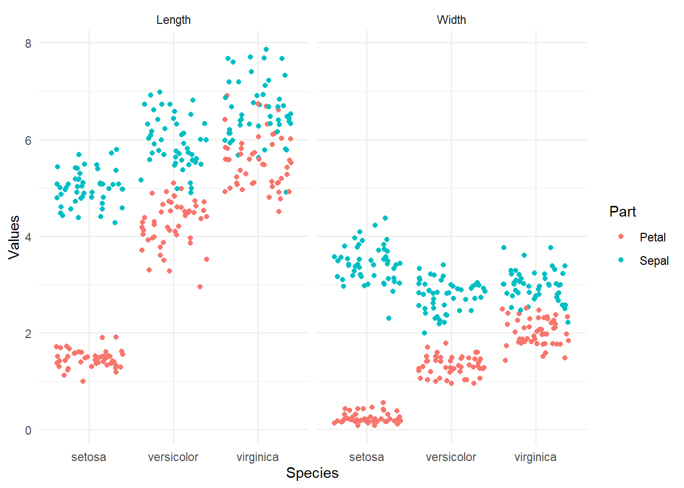
9.2 pivot_longer()
A common problem is a dataset where some of the column names are not names of variables, but values of a variable
- pivot_longer(data, cols, names_to, values_to)
- cols : columns to pivot into longer format
- names_to : A string specifying the name of the column to create from the data stored in the column names of data
- values_to : A string specifying the name of the column to create from the data stored in cell values
## # A tibble: 3 x 3
##   country     `1999` `2000`
## * <chr>        <int>  <int>
## 1 Afghanistan    745   2666
## 2 Brazil       37737  80488
## 3 China 212258 213766## # A tibble: 6 x 3
## country year cases
## <chr> <chr> <int>
## 1 Afghanistan 1999 745
## 2 Afghanistan 2000 2666
## 3 Brazil 1999 37737
## 4 Brazil 2000 80488
## 5 China 1999 212258
## 6 China 2000 2137669.2.1 Exercise 1
relig_income is a tibble in tidyr which contains the result of religion and income survey
## # A tibble: 18 x 11
##    religion            `<$10k` `$10-20k` `$20-30k` `$30-40k` `$40-50k` `$50-75k` `$75-100k` `$100-150k` `>150k` `Don't know/refus~
##    <chr>                 <dbl>     <dbl>     <dbl>     <dbl>     <dbl>     <dbl>      <dbl>       <dbl>   <dbl>              <dbl>
##  1 Agnostic                 27        34        60        81        76       137        122         109      84                 96
##  2 Atheist                  12        27        37        52        35        70         73          59      74                 76
##  3 Buddhist                 27        21        30        34        33        58         62          39      53                 54
##  4 Catholic                418       617       732       670       638      1116        949         792     633               1489
##  5 Don’t know/refused       15        14        15        11        10        35         21          17      18                116
##  6 Evangelical Prot        575       869      1064       982       881      1486        949         723     414               1529
##  7 Hindu                     1         9         7         9        11        34         47          48      54                 37
##  8 Historically Black~     228       244       236       238       197       223        131          81      78                339
##  9 Jehovah's Witness        20        27        24        24        21        30         15          11       6                 37
## 10 Jewish                   19        19        25        25        30        95         69          87     151                162
## 11 Mainline Prot           289       495       619       655       651      1107        939         753     634               1328
## 12 Mormon                   29        40        48        51        56       112         85          49      42                 69
## 13 Muslim                    6         7         9        10         9        23         16           8       6                 22
## 14 Orthodox                 13        17        23        32        32        47         38          42      46                 73
## 15 Other Christian           9         7        11        13        13        14         18          14      12                 18
## 16 Other Faiths             20        33        40        46        49        63         46          40      41                 71
## 17 Other World Religi~       5         2         3         4         2         7          3           4       4                  8
## 18 Unaffiliated 217 299 374 365 341 528 407 321 258 597## # A tibble: 180 x 3
## religion income value
## <chr> <chr> <dbl>
## 1 Agnostic <$10k 27
## 2 Agnostic $10-20k 34
## 3 Agnostic $20-30k 60
## 4 Agnostic $30-40k 81
## 5 Agnostic $40-50k 76
## 6 Agnostic $50-75k 137
## 7 Agnostic $75-100k 122
## 8 Agnostic $100-150k 109
## 9 Agnostic >150k 84
## 10 Agnostic Don't know/refused 96
## # ... with 170 more rows9.2.2 Exercise 2
stocks <- tibble(
  time = as.Date('2009-01-01') + 0:1,
  Stock_X = c(1000,1200),
  Stock_Y = c(900,1000),
  Stock_Z = c(1400,1000)
)## # A tibble: 2 x 4
## time Stock_X Stock_Y Stock_Z
## <date> <dbl> <dbl> <dbl>
## 1 2009-01-01 1000 900 1400
## 2 2009-01-02 1200 1000 1000## # A tibble: 6 x 3
## time stock price
## <date> <chr> <dbl>
## 1 2009-01-01 Stock_X 1000
## 2 2009-01-01 Stock_Y 900
## 3 2009-01-01 Stock_Z 1400
## 4 2009-01-02 Stock_X 1200
## 5 2009-01-02 Stock_Y 1000
## 6 2009-01-02 Stock_Z 10009.2.3 Exercise 3
## # A tibble: 317 x 79
##    artist track date.entered   wk1   wk2   wk3   wk4   wk5   wk6   wk7   wk8   wk9  wk10  wk11  wk12  wk13  wk14  wk15  wk16  wk17
##    <chr>  <chr> <date>       <dbl> <dbl> <dbl> <dbl> <dbl> <dbl> <dbl> <dbl> <dbl> <dbl> <dbl> <dbl> <dbl> <dbl> <dbl> <dbl> <dbl>
##  1 2 Pac  Baby~ 2000-02-26      87    82    72    77    87    94    99    NA    NA    NA    NA    NA    NA    NA    NA    NA    NA
##  2 2Ge+h~ The ~ 2000-09-02      91    87    92    NA    NA    NA    NA    NA    NA    NA    NA    NA    NA    NA    NA    NA    NA
##  3 3 Doo~ Kryp~ 2000-04-08      81    70    68    67    66    57    54    53    51    51    51    51    47    44    38    28    22
##  4 3 Doo~ Loser 2000-10-21      76    76    72    69    67    65    55    59    62    61    61    59    61    66    72    76    75
##  5 504 B~ Wobb~ 2000-04-15      57    34    25    17    17    31    36    49    53    57    64    70    75    76    78    85    92
##  6 98^0   Give~ 2000-08-19      51    39    34    26    26    19     2     2     3     6     7    22    29    36    47    67    66
##  7 A*Tee~ Danc~ 2000-07-08      97    97    96    95   100    NA    NA    NA    NA    NA    NA    NA    NA    NA    NA    NA    NA
##  8 Aaliy~ I Do~ 2000-01-29      84    62    51    41    38    35    35    38    38    36    37    37    38    49    61    63    62
##  9 Aaliy~ Try ~ 2000-03-18      59    53    38    28    21    18    16    14    12    10     9     8     6     1     2     2     2
## 10 Adams~ Open~ 2000-08-26      76    76    74    69    68    67    61    58    57    59    66    68    61    67    59    63    67
## # ... with 307 more rows, and 59 more variables: wk18 <dbl>, wk19 <dbl>, wk20 <dbl>, wk21 <dbl>, wk22 <dbl>, wk23 <dbl>,
## #   wk24 <dbl>, wk25 <dbl>, wk26 <dbl>, wk27 <dbl>, wk28 <dbl>, wk29 <dbl>, wk30 <dbl>, wk31 <dbl>, wk32 <dbl>, wk33 <dbl>,
## #   wk34 <dbl>, wk35 <dbl>, wk36 <dbl>, wk37 <dbl>, wk38 <dbl>, wk39 <dbl>, wk40 <dbl>, wk41 <dbl>, wk42 <dbl>, wk43 <dbl>,
## #   wk44 <dbl>, wk45 <dbl>, wk46 <dbl>, wk47 <dbl>, wk48 <dbl>, wk49 <dbl>, wk50 <dbl>, wk51 <dbl>, wk52 <dbl>, wk53 <dbl>,
## #   wk54 <dbl>, wk55 <dbl>, wk56 <dbl>, wk57 <dbl>, wk58 <dbl>, wk59 <dbl>, wk60 <dbl>, wk61 <dbl>, wk62 <dbl>, wk63 <dbl>,
## #   wk64 <dbl>, wk65 <dbl>, wk66 <lgl>, wk67 <lgl>, wk68 <lgl>, wk69 <lgl>, wk70 <lgl>, wk71 <lgl>, wk72 <lgl>, wk73 <lgl>,
## #   wk74 <lgl>, wk75 <lgl>, wk76 <lgl>
billboard %>%
pivot_longer(
cols = starts_with("wk"),
names_to = "week",
values_to = "rank",
values_drop_na = TRUE
)## # A tibble: 5,307 x 5
## artist track date.entered week rank
## <chr> <chr> <date> <chr> <dbl>
## 1 2 Pac Baby Don't Cry (Keep... 2000-02-26 wk1 87
## 2 2 Pac Baby Don't Cry (Keep... 2000-02-26 wk2 82
## 3 2 Pac Baby Don't Cry (Keep... 2000-02-26 wk3 72
## 4 2 Pac Baby Don't Cry (Keep... 2000-02-26 wk4 77
## 5 2 Pac Baby Don't Cry (Keep... 2000-02-26 wk5 87
## 6 2 Pac Baby Don't Cry (Keep... 2000-02-26 wk6 94
## 7 2 Pac Baby Don't Cry (Keep... 2000-02-26 wk7 99
## 8 2Ge+her The Hardest Part Of ... 2000-09-02 wk1 91
## 9 2Ge+her The Hardest Part Of ... 2000-09-02 wk2 87
## 10 2Ge+her The Hardest Part Of ... 2000-09-02 wk3 92
## # ... with 5,297 more rows9.3 pivot_wider()
we use it when an observation is scattered across multiple rows
- pivot_wider(data, names_from, values_from)
- names_from : A string specifying the name of the column to get the name of the output column
- values_from : A string specifying the name of the column to get the cell values from
## # A tibble: 12 x 4
##    country      year type            count
##    <chr>       <int> <chr>           <int>
##  1 Afghanistan  1999 cases             745
##  2 Afghanistan  1999 population   19987071
##  3 Afghanistan  2000 cases            2666
##  4 Afghanistan  2000 population   20595360
##  5 Brazil       1999 cases           37737
##  6 Brazil       1999 population  172006362
##  7 Brazil       2000 cases           80488
##  8 Brazil       2000 population  174504898
##  9 China        1999 cases          212258
## 10 China        1999 population 1272915272
## 11 China        2000 cases          213766
## 12 China 2000 population 1280428583## # A tibble: 6 x 4
## country year cases population
## <chr> <int> <int> <int>
## 1 Afghanistan 1999 745 19987071
## 2 Afghanistan 2000 2666 20595360
## 3 Brazil 1999 37737 172006362
## 4 Brazil 2000 80488 174504898
## 5 China 1999 212258 1272915272
## 6 China 2000 213766 12804285839.4 separate()
separate() separates a single column into multiple columns. It will split values wherever it sees a non-alphanumeric characters
## # A tibble: 6 x 3
## country year rate
## * <chr> <int> <chr>
## 1 Afghanistan 1999 745/19987071
## 2 Afghanistan 2000 2666/20595360
## 3 Brazil 1999 37737/172006362
## 4 Brazil 2000 80488/174504898
## 5 China 1999 212258/1272915272
## 6 China 2000 213766/1280428583By default, any non-alphanumeric character will be a delimiter
## # A tibble: 6 x 4
## country year cases population
## <chr> <int> <chr> <chr>
## 1 Afghanistan 1999 745 19987071
## 2 Afghanistan 2000 2666 20595360
## 3 Brazil 1999 37737 172006362
## 4 Brazil 2000 80488 174504898
## 5 China 1999 212258 1272915272
## 6 China 2000 213766 1280428583you can specify your own delimiter using sep
## # A tibble: 6 x 4
## country year cases population
## <chr> <int> <chr> <chr>
## 1 Afghanistan 1999 745 19987071
## 2 Afghanistan 2000 2666 20595360
## 3 Brazil 1999 37737 172006362
## 4 Brazil 2000 80488 174504898
## 5 China 1999 212258 1272915272
## 6 China 2000 213766 1280428583convert = TRUE will convert to better type(chr -> int)
## # A tibble: 6 x 4
##   country      year  cases population
##   <chr>       <int>  <int>      <int>
## 1 Afghanistan  1999    745   19987071
## 2 Afghanistan  2000   2666   20595360
## 3 Brazil       1999  37737  172006362
## 4 Brazil       2000  80488  174504898
## 5 China        1999 212258 1272915272
## 6 China 2000 213766 1280428583separate() will interpret the integers as positions to split at
## # A tibble: 6 x 4
##   country     century year  rate
##   <chr>       <chr>   <chr> <chr>
## 1 Afghanistan 19      99    745/19987071
## 2 Afghanistan 20      00    2666/20595360
## 3 Brazil      19      99    37737/172006362
## 4 Brazil      20      00    80488/174504898
## 5 China       19      99    212258/1272915272
## 6 China       20      00    213766/1280428583
9.5 Unite()
unite() combines multiple columns into a single column
## # A tibble: 6 x 4
##   country     century year  rate
## * <chr>       <chr>   <chr> <chr>
## 1 Afghanistan 19      99    745/19987071
## 2 Afghanistan 20      00    2666/20595360
## 3 Brazil      19      99    37737/172006362
## 4 Brazil      20      00    80488/174504898
## 5 China       19      99    212258/1272915272
## 6 China       20      00    213766/1280428583
By default, unite() will place an underscore(_)
## # A tibble: 6 x 3
##   country     new   rate
##   <chr>       <chr> <chr>
## 1 Afghanistan 19_99 745/19987071
## 2 Afghanistan 20_00 2666/20595360
## 3 Brazil      19_99 37737/172006362
## 4 Brazil      20_00 80488/174504898
## 5 China       19_99 212258/1272915272
## 6 China 20_00 213766/1280428583## # A tibble: 6 x 3
## country new rate
## <chr> <chr> <chr>
## 1 Afghanistan 1999 745/19987071
## 2 Afghanistan 2000 2666/20595360
## 3 Brazil 1999 37737/172006362
## 4 Brazil 2000 80488/174504898
## 5 China 1999 212258/1272915272
## 6 China 2000 213766/1280428583