Chapter 6 Base R
10월 1일 목요일, 202AIE17 송채은
6.2 Functions
a function is a block of codes that is used to perform a single task when the function is called
- A function requires
- arguments : whose values will be used if the function is called
- body : which is a group of R expressions contained in a curly brace ({ and })
- Functions are a fundamental building block of R
- Packages are a collection of functions made by others
- our job is to build a pipeline of data flow by connecting many available functions
1. An Example of Functions
## [1] 2.5mean() will not work with NA
## [1] NAWhen na.rm = TRUE, NA will be removed before computation
## [1] 2.3333332. User-Defined Functions
## [1] 0.41582473. Exercise on functions
## [1] 2.8209146.3 Operators
## [1] FALSE## [1] TRUE## [1] TRUE## [1] FALSE6.4 Data Structure
R has base structures and base data structures can be organized by their dimensionality element를 찾기 위한 Index의 갯수가 1개(1D), 2개(2D), n개(nD)
6.5 Vectors
Atomic Vectors(homogeneous)
- All elements of an atomic vector must be the same type and usually created with c()
- Logical (TRUE or FALSE) 논리
- integer 정수
- double 실수
- character 문자
- complex 복소수
- raw
Lists (heterogeneous) their elements can be of any type and lists are created by list()
6.5.1 Vector Has Three Properties
1. Type
typeof() returns the type of an object
## [1] "double"2. Length
length() returns the number of elements in a vector
## [1] 33. Attributes
attr() or attributes() returns additional arbitrary metadata
## NULL## [1] "x" "y" "z"modifying existing names
## l m n
## 1 2 3
names are attributes
## $names
## [1] "l" "m" "n"## mpg cyl disp hp drat wt qsec vs am gear carb
## Mazda RX4 21.0 6 160 110 3.90 2.620 16.46 0 1 4 4
## Mazda RX4 Wag 21.0 6 160 110 3.90 2.875 17.02 0 1 4 4
## Datsun 710 22.8 4 108 93 3.85 2.320 18.61 1 1 4 1
## Hornet 4 Drive 21.4 6 258 110 3.08 3.215 19.44 1 0 3 1
## Hornet Sportabout 18.7 8 360 175 3.15 3.440 17.02 0 0 3 2
## Valiant 18.1 6 225 105 2.76 3.460 20.22 1 0 3 1## $names
## [1] "mpg" "cyl" "disp" "hp" "drat" "wt" "qsec" "vs" "am" "gear" "carb"
##
## $row.names
## [1] "Mazda RX4" "Mazda RX4 Wag" "Datsun 710" "Hornet 4 Drive" "Hornet Sportabout"
## [6] "Valiant" "Duster 360" "Merc 240D" "Merc 230" "Merc 280"
## [11] "Merc 280C" "Merc 450SE" "Merc 450SL" "Merc 450SLC" "Cadillac Fleetwood"
## [16] "Lincoln Continental" "Chrysler Imperial" "Fiat 128" "Honda Civic" "Toyota Corolla"
## [21] "Toyota Corona" "Dodge Challenger" "AMC Javelin" "Camaro Z28" "Pontiac Firebird"
## [26] "Fiat X1-9" "Porsche 914-2" "Lotus Europa" "Ford Pantera L" "Ferrari Dino"
## [31] "Maserati Bora" "Volvo 142E"
##
## $class
## [1] "data.frame"6.5.2 Type Conversion
All elements of a vector must belong to the same base data type. If that is not true, R will automatically force it by type conversion
## [1] "4" "7" "23.5" "76.2" "80" "rrt"## [1] "character"Functions can automatically convert data type TRUE = 1, FALSE = 2
## [1] 2can convert data type with as.character(), as.double(), as.integer(), and as.logical()
## [1] 1 2 3## [1] "1" "2" "3"6.5.3 Generate a vector
## [1] 1 2 3 4 5c() also combine vectors
## [1] 1 2 3 4 5 6k:n generates a vector whose elements are the sequence of numbers from k to n
## [1] 1 2 3 4 5 6 7 8 9 10seq() generates regular sequence seq(from, to)
## [1] 1 2 3 4 5 6 7 8 9 10seq(from, to, by)
## [1] 1 3 5 7 9rep(x, times) replicates the values in x multiple times (x can be a number or vector)
## [1] 1 1 1 1 1## [1] 1 2 1 2 1 2 1 2 1 2## [1] 1 1 1 1 1 2 2 2 2 2## [1] 1.05430020 -0.70747447 -0.32920300 -0.46654981 0.25314117 1.43733792 0.10544477 -1.05807539 0.43049233 -1.98590939
## [11] 1.49579578 -0.04953275 -0.95942917 -0.65197615 0.69324827 -0.72920304 -0.86872850 0.87616007 0.70878155 -0.29516434
## [21] -0.14410707 0.92548801 -0.44549329 0.19453602 -1.60115211 1.39350959 3.32606250 -0.79648802 -1.30996456 -0.46003636
## [31] -0.53669533 0.82104467 1.78821753 -1.97608002 1.52531876 -0.25585319 1.21006074 1.95607085 0.04230925 0.46803578
## [41] 2.01670378 1.19368046 1.20120153 -0.49669237 -0.18918695 -0.42362620 0.41901524 -0.39265277 -0.90423529 -1.68525596
## [51] -0.99853779 -0.05946837 -0.12272501 1.19990084 -0.25277591 0.06012662 -1.08792087 0.76878385 -0.06246595 -2.07270115
## [61] -1.31755700 -0.89706424 0.34031477 0.90086963 -0.11628450 -0.24003826 -1.18040086 -0.24690402 -0.83260657 -1.00306421
## [71] -0.30850349 -0.34659285 0.43716883 -2.36077103 -0.23116019 1.87449880 1.38009796 0.95581840 -0.08384473 0.26942021
## [81] 1.08039932 0.40561762 0.15912815 1.13572438 0.10386879 0.86585554 0.79493803 -0.43080560 0.77649804 -0.32221706
## [91] 1.50550855 0.32032912 0.24727775 -0.82197481 -1.42758024 1.10942098 1.39620746 0.08895578 0.46403878 -0.54669577## `stat_bin()` using `bins = 30`. Pick better value with `binwidth`.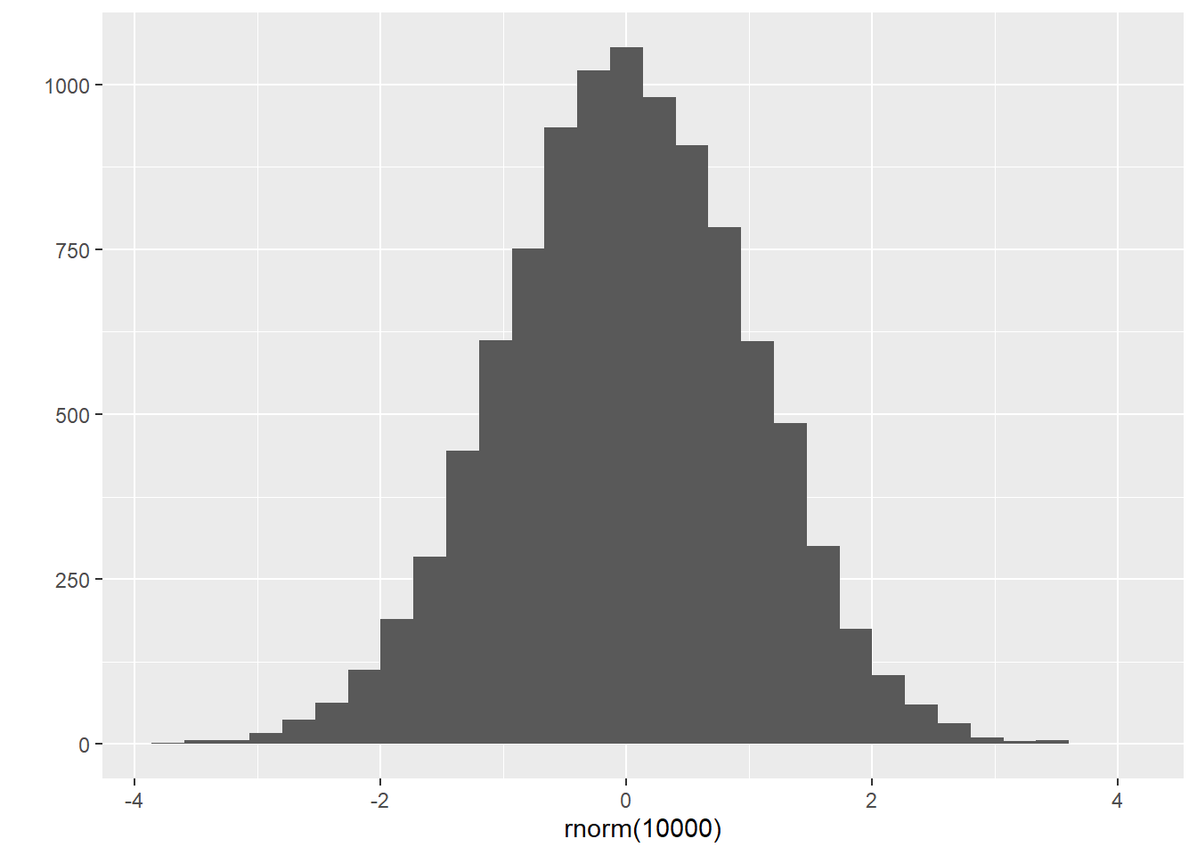
runif(n, min, max) generates a vector of n random samples from a uniform distribution whose limits are min and max
##   [1] 0.472724686 0.307018266 0.720369834 0.565719134 0.260214073 0.291630986 0.882164101 0.051605914 0.455890893 0.165143798
##  [11] 0.851892580 0.040269077 0.366332942 0.673759001 0.057252024 0.706318196 0.217254666 0.262953555 0.404861972 0.751126933
##  [21] 0.126246933 0.472105791 0.134025459 0.689038690 0.783065907 0.164032331 0.101259435 0.565697048 0.060336350 0.765656369
##  [31] 0.511318344 0.724996882 0.869950069 0.912974228 0.905732265 0.743389372 0.374935023 0.532313017 0.094557391 0.724723988
##  [41] 0.379362820 0.882813673 0.996418042 0.331454388 0.511362910 0.083599654 0.792371807 0.218166791 0.266773995 0.006076652
##  [51] 0.064438633 0.565171633 0.112191624 0.796797916 0.464214930 0.866476413 0.754352485 0.269016077 0.259146014 0.664641577
##  [61] 0.988021544 0.914366963 0.661401265 0.768460279 0.666844471 0.408162299 0.735091421 0.749441098 0.768186237 0.223100694
##  [71] 0.946561704 0.962713837 0.938126939 0.832991195 0.182621158 0.988980525 0.530086909 0.550687216 0.148937527 0.271781892
##  [81] 0.011120157 0.151779840 0.667246365 0.367090994 0.024391824 0.755280936 0.867969546 0.033019193 0.211942921 0.705608915
## [91] 0.724538469 0.230190331 0.617799667 0.790173059 0.995027459 0.348505143 0.956797696 0.023629957 0.851972289 0.025694436## `stat_bin()` using `bins = 30`. Pick better value with `binwidth`.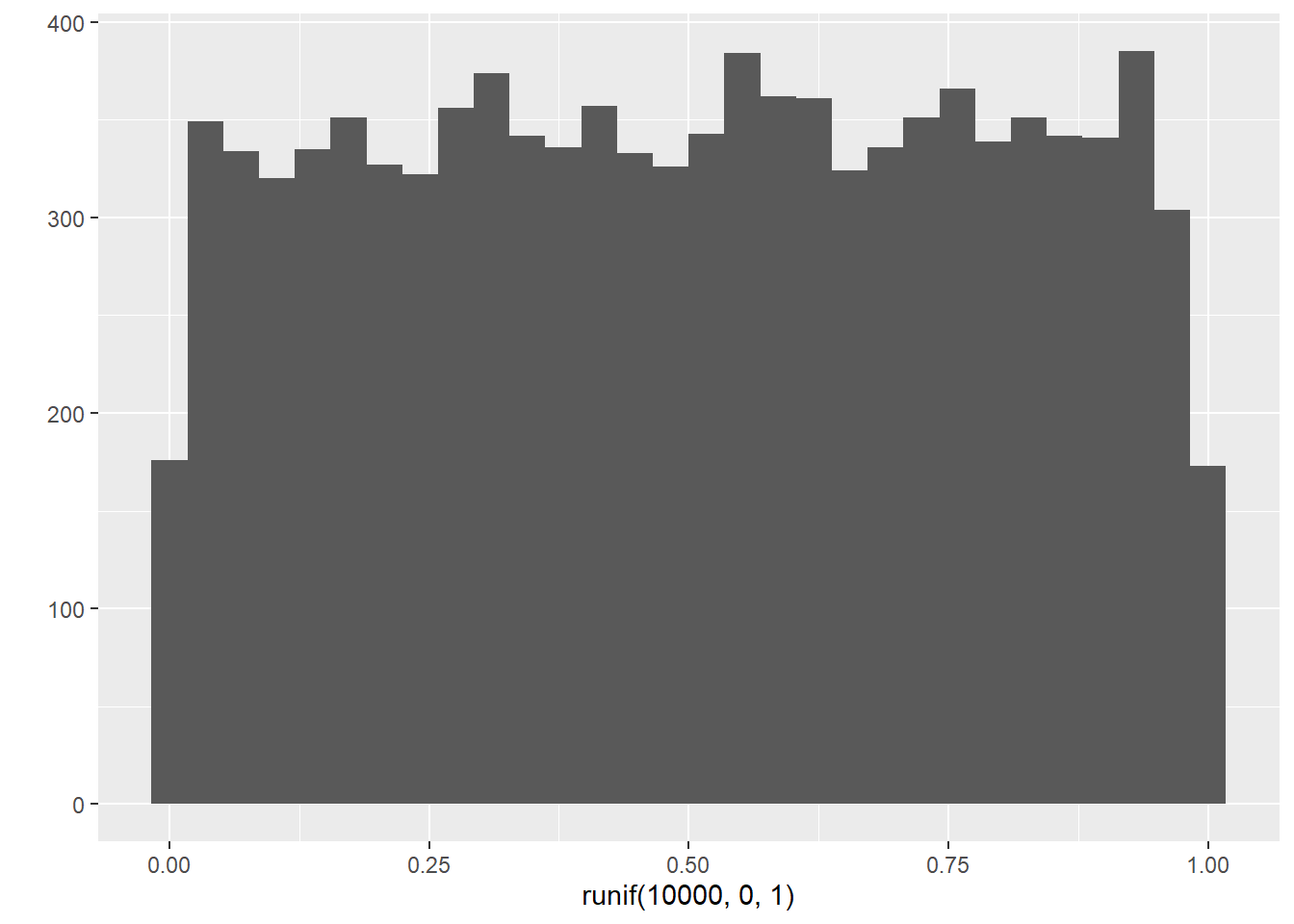
6.5.4 Indexing or subsetting a Vector
access a particular element of a vector through an index between square brackets or indexing (subsetting) operator
1. Positive integers
return elements at the specified positions
## [1] 4 22. Negative integers
omit elements at the specified positions
## [1] 3 5 6 73. Logical vectors
select elements where the corresponding logical value is TRUE
## [1] 2 3 6 7## [1] FALSE FALSE TRUE TRUE TRUE TRUEThis is called a logical indexing
## [1] 4 5 6 7## [1] 4v1 %in% v2 returns a logical vector indicating whether the elements of v1 are included in v2
## [1] FALSE TRUE TRUE## [1] 1 2 3 4 5## [1] 1 2 100 4 5## [1] 100 2 100 4 100## [1] 1 2 3 NA 5 6 NAis.na indicates which elements are missing
## [1] FALSE FALSE FALSE TRUE FALSE FALSE TRUETRUE and FALSE will be converted into 1 and 0
## [1] 2## [1] TRUE TRUE TRUE FALSE TRUE TRUE FALSE## [1] 5## [1] 1 2 3 999 5 6 999create a vector with names
## x y z
## 1 2 3
named vector can be indexed using their names
## x z
## 1 3
R uses a “recycling rule” by repeating the shorter vector
## [1] 1 3## [1] 14 15 16 176.5.5 Arrange a vector
sort() sorts ascending order
## [1] 4 5 6sorts into descending order
## [1] 6 5 4rev() provides a reversed version of its argument
## [1] 4 6 5rank() returns the sample ranks of the elements in a vector
## [1] 2 3 1order() returns a permutation which rearranges 1) first sorts a vector in ascending order to produce c(4,5,6) 2) and returns the indices of the sorted element in the original vector
## [1] 3 1 2## [1] 4 5 6## mpg cyl disp hp drat wt qsec vs am gear carb
## Cadillac Fleetwood 10.4 8 472 205 2.93 5.250 17.98 0 0 3 4
## Lincoln Continental 10.4 8 460 215 3.00 5.424 17.82 0 0 3 4
## Camaro Z28 13.3 8 350 245 3.73 3.840 15.41 0 0 3 4
## Duster 360 14.3 8 360 245 3.21 3.570 15.84 0 0 3 4
## Chrysler Imperial 14.7 8 440 230 3.23 5.345 17.42 0 0 3 4
## Maserati Bora 15.0 8 301 335 3.54 3.570 14.60 0 1 5 86.5.6 Vectorization of Functions
Many R functions can be applied to a vector of values producing an equal-sized vector of result
## [1] 1 2 5## [1] 1 4 9## [1] 14 7 7 9R uses a “recycling rule” by repeating the shorter vector
## [1] 14 7 16 9mean will be subtracted from every element of v1
## [1] -1.5 -0.5 0.5 1.56.5.7 Some more functions
table() creates a frequency table
## a
## 1 2 3 4
## 2 3 3 5
unique() returns a vector of unique elements
## [1] 1 2 3 4By default, mean() produces NA when there’s NAs in a vector
## [1] NAna.rm = TRUE removes NAs before computation
## [1] 2.758. Generating Sequences
creating a vector containing integers between 1 and 10
## [1] 1 2 3 4 5 6 7 8 9 10## [1] 5 4 3 2 1 0## [1] 1.0 1.5 2.0 2.5 3.0## [1] 1.0 1.5 2.0 2.5 3.0rep() replicates each term in formula
## [1] 5 5 5## [1] 1 2 1 2 1 2## [1] 1 1 1 2 2 2gl(k,n) generates sequences involving factors + k : the number of levels + n : the number of repetitions
##  [1] 1 1 1 2 2 2 3 3 3 4 4 4 5 5 5
## Levels: 1 2 3 4 5
9. Exercise on vectors
## [1] 32Calculate the mean of a using sum() and length() functions
## [1] 20.09062## [1] 20.09062Calculate the variance of a using sd() function
## [1] 36.3241Calculate the variance of a using var() function
## [1] 36.3241## [1] 0.15088482 0.15088482 0.44954345 0.21725341 -0.23073453 -0.33028740 -0.96078893 0.71501778 0.44954345 -0.14777380
## [11] -0.38006384 -0.61235388 -0.46302456 -0.81145962 -1.60788262 -1.60788262 -0.89442035 2.04238943 1.71054652 2.29127162
## [21] 0.23384555 -0.76168319 -0.81145962 -1.12671039 -0.14777380 1.19619000 0.98049211 1.71054652 -0.71190675 -0.06481307
## [31] -0.84464392 0.21725341Use scale() function to standardize a and compare the results with your manual calculation
##              [,1]
##  [1,]  0.15088482
##  [2,]  0.15088482
##  [3,]  0.44954345
##  [4,]  0.21725341
##  [5,] -0.23073453
##  [6,] -0.33028740
##  [7,] -0.96078893
##  [8,]  0.71501778
##  [9,]  0.44954345
## [10,] -0.14777380
## [11,] -0.38006384
## [12,] -0.61235388
## [13,] -0.46302456
## [14,] -0.81145962
## [15,] -1.60788262
## [16,] -1.60788262
## [17,] -0.89442035
## [18,]  2.04238943
## [19,]  1.71054652
## [20,]  2.29127162
## [21,]  0.23384555
## [22,] -0.76168319
## [23,] -0.81145962
## [24,] -1.12671039
## [25,] -0.14777380
## [26,]  1.19619000
## [27,]  0.98049211
## [28,]  1.71054652
## [29,] -0.71190675
## [30,] -0.06481307
## [31,] -0.84464392
## [32,]  0.21725341
## attr(,"scaled:center")
## [1] 20.09062
## attr(,"scaled:scale")
## [1] 6.026948
Calculate the difference between the largest and smallest numbers in a
## [1] 23.5## [1] 23.5Normalize the vector
##  [1] 0.4510638 0.4510638 0.5276596 0.4680851 0.3531915 0.3276596 0.1659574 0.5957447 0.5276596 0.3744681 0.3148936 0.2553191
## [13] 0.2936170 0.2042553 0.0000000 0.0000000 0.1829787 0.9361702 0.8510638 1.0000000 0.4723404 0.2170213 0.2042553 0.1234043
## [25] 0.3744681 0.7191489 0.6638298 0.8510638 0.2297872 0.3957447 0.1957447 0.4680851## `stat_bin()` using `bins = 30`. Pick better value with `binwidth`.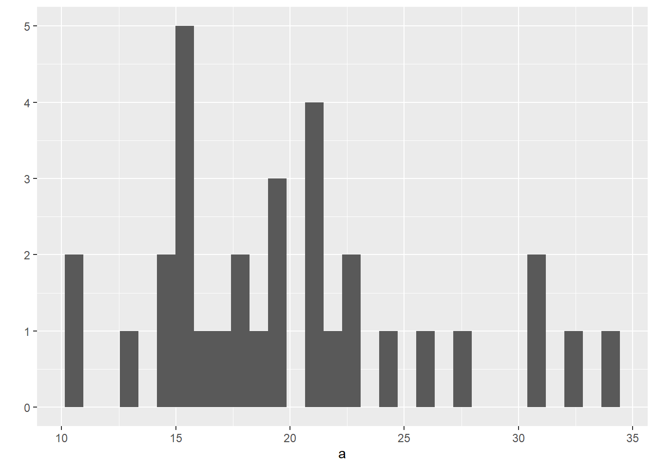
To set aesthetics, wrap in I()
## `stat_bin()` using `bins = 30`. Pick better value with `binwidth`.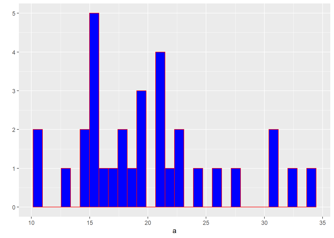
How many elements in a are larger than 20?
##  [1]  TRUE  TRUE  TRUE  TRUE FALSE FALSE FALSE  TRUE  TRUE FALSE FALSE FALSE FALSE FALSE FALSE FALSE FALSE  TRUE  TRUE  TRUE  TRUE
## [22] FALSE FALSE FALSE FALSE  TRUE  TRUE  TRUE FALSE FALSE FALSE  TRUE
within the subsetting operator (i.e., []) will create a vector with elements larger than 20
## [1] 21.0 21.0 22.8 21.4 24.4 22.8 32.4 30.4 33.9 21.5 27.3 26.0 30.4 21.4## [1] 14How many elements in a are larger than 20?
## [1] 14## # A tibble: 6 x 9
## city year month sales volume median listings inventory date
## <chr> <int> <int> <dbl> <dbl> <dbl> <dbl> <dbl> <dbl>
## 1 Abilene 2000 1 72 5380000 71400 701 6.3 2000
## 2 Abilene 2000 2 98 6505000 58700 746 6.6 2000.
## 3 Abilene 2000 3 130 9285000 58100 784 6.8 2000.
## 4 Abilene 2000 4 98 9730000 68600 785 6.9 2000.
## 5 Abilene 2000 5 141 10590000 67300 794 6.8 2000.
## 6 Abilene 2000 6 156 13910000 66900 780 6.6 2000.## [1] 8602## [1] 616## [1] 118955.8## [1] 128131.4