Chapter 5 R markdown
9월 24일 목요일, 202AIE17 송채은
What is R markdown documents?
R markdown document(.Rmd) allows us to create a report in a variety of formats (ex.html, pdf, word, slides, interactive documents) that includes your codes, results, and texts
- When you render an R markdown document using the render() function
- knitr : executes all code chunks in an R markdown document to create a new markdown document (.md)
- pandoc : converts a markdown document to the final format
An R markdown document has YAML header, text, code chunks
5.1 Problem 1
## # A tibble: 6 x 11
##   manufacturer model displ  year   cyl trans      drv     cty   hwy fl    class
##   <chr>        <chr> <dbl> <int> <int> <chr>      <chr> <int> <int> <chr> <chr>
## 1 audi         a4      1.8  1999     4 auto(l5)   f        18    29 p     compact
## 2 audi         a4      1.8  1999     4 manual(m5) f        21    29 p     compact
## 3 audi         a4      2    2008     4 manual(m6) f        20    31 p     compact
## 4 audi         a4      2    2008     4 auto(av)   f        21    30 p     compact
## 5 audi         a4      2.8  1999     6 auto(l5)   f        16    26 p     compact
## 6 audi a4 2.8 1999 6 manual(m5) f 18 26 p compactggplot(mpg, aes(hwy, fill = drv)) +
geom_histogram(alpha = 0.5) +
theme_minimal() +
labs(title = "Histogram",
subtitle = "Histogram of Highway Mile Per Gallon",
caption = "Source: mpg")## `stat_bin()` using `bins = 30`. Pick better value with `binwidth`.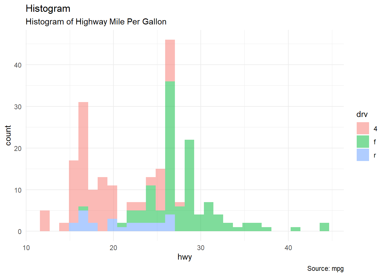
5.2 Problem 2
ggplot(mpg, aes(hwy, fill = drv)) +
  geom_histogram(alpha = 0.5) +
  facet_grid(rows = vars(drv)) +
  theme_minimal() +
  labs(title = "Histogram using facet_grid()",
       subtitle = "Histogram of Highway Mile Per Gallon",
       caption = "Source: mpg")
## `stat_bin()` using `bins = 30`. Pick better value with `binwidth`.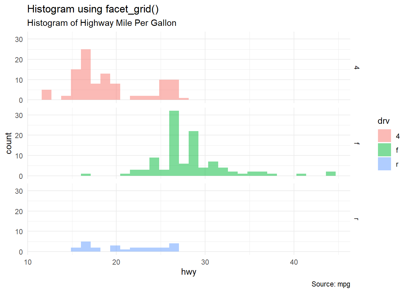
5.3 Problem 3
## # A tibble: 6 x 28
##     PID county state  area poptotal popdensity popwhite popblack popamerindian popasian popother percwhite percblack percamerindan
##   <int> <chr>  <chr> <dbl>    <int>      <dbl>    <int>    <int>         <int>    <int>    <int>     <dbl>     <dbl>         <dbl>
## 1   561 ADAMS  IL    0.052    66090      1271.    63917     1702            98      249      124      96.7     2.58          0.148
## 2   562 ALEXA~ IL    0.014    10626       759      7054     3496            19       48        9      66.4    32.9           0.179
## 3   563 BOND   IL    0.022    14991       681.    14477      429            35       16       34      96.6     2.86          0.233
## 4   564 BOONE  IL    0.017    30806      1812.    29344      127            46      150     1139      95.3     0.412         0.149
## 5   565 BROWN  IL    0.018     5836       324.     5264      547            14        5        6      90.2     9.37          0.240
## 6   566 BUREAU IL    0.05     35688       714.    35157       50            65      195      221      98.5     0.140         0.182
## # ... with 14 more variables: percasian <dbl>, percother <dbl>, popadults <int>, perchsd <dbl>, percollege <dbl>, percprof <dbl>,
## #   poppovertyknown <int>, percpovertyknown <dbl>, percbelowpoverty <dbl>, percchildbelowpovert <dbl>, percadultpoverty <dbl>,
## # percelderlypoverty <dbl>, inmetro <int>, category <chr>ggplot(midwest, aes(area, poptotal)) +
geom_point(aes(color = state, size = popdensity), alpha = 0.4) +
geom_smooth(method="loess", se=FALSE) +
xlim(c(0, 0.1)) +
ylim(c(0, 500000)) +
theme_classic() +
labs(title = "Scatterplot",
subtitle="Area Vs Population",
caption = "Source: midwest",
x = "Area",
y = "Population")## `geom_smooth()` using formula 'y ~ x'## Warning: Removed 15 rows containing non-finite values (stat_smooth).## Warning: Removed 15 rows containing missing values (geom_point).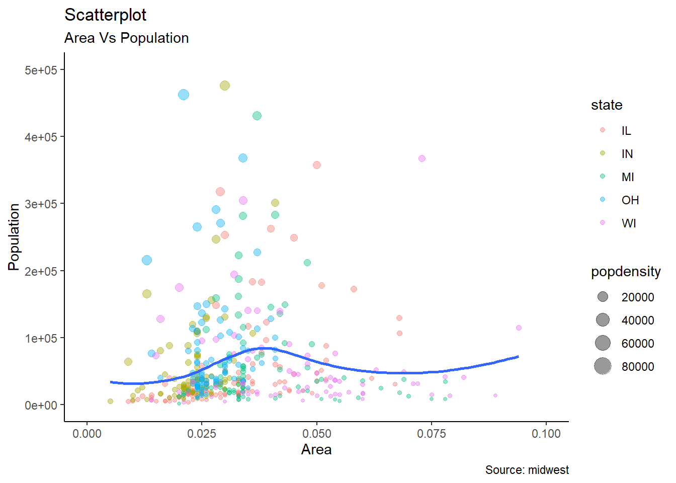
5.4 Problem 4
##   Sepal.Length Sepal.Width Petal.Length Petal.Width Species
## 1          5.1         3.5          1.4         0.2  setosa
## 2          4.9         3.0          1.4         0.2  setosa
## 3          4.7         3.2          1.3         0.2  setosa
## 4          4.6         3.1          1.5         0.2  setosa
## 5          5.0         3.6          1.4         0.2  setosa
## 6 5.4 3.9 1.7 0.4 setosaggplot(iris, aes(Sepal.Length, Sepal.Width)) +
geom_point(aes(color = Species, shape = Species), size = 6, alpha = 0.5) +
theme_minimal() +
labs(title = "Scatterplot",
subtitle="Sepal.Length Vs Sepal.Width",
caption = "Source: iris")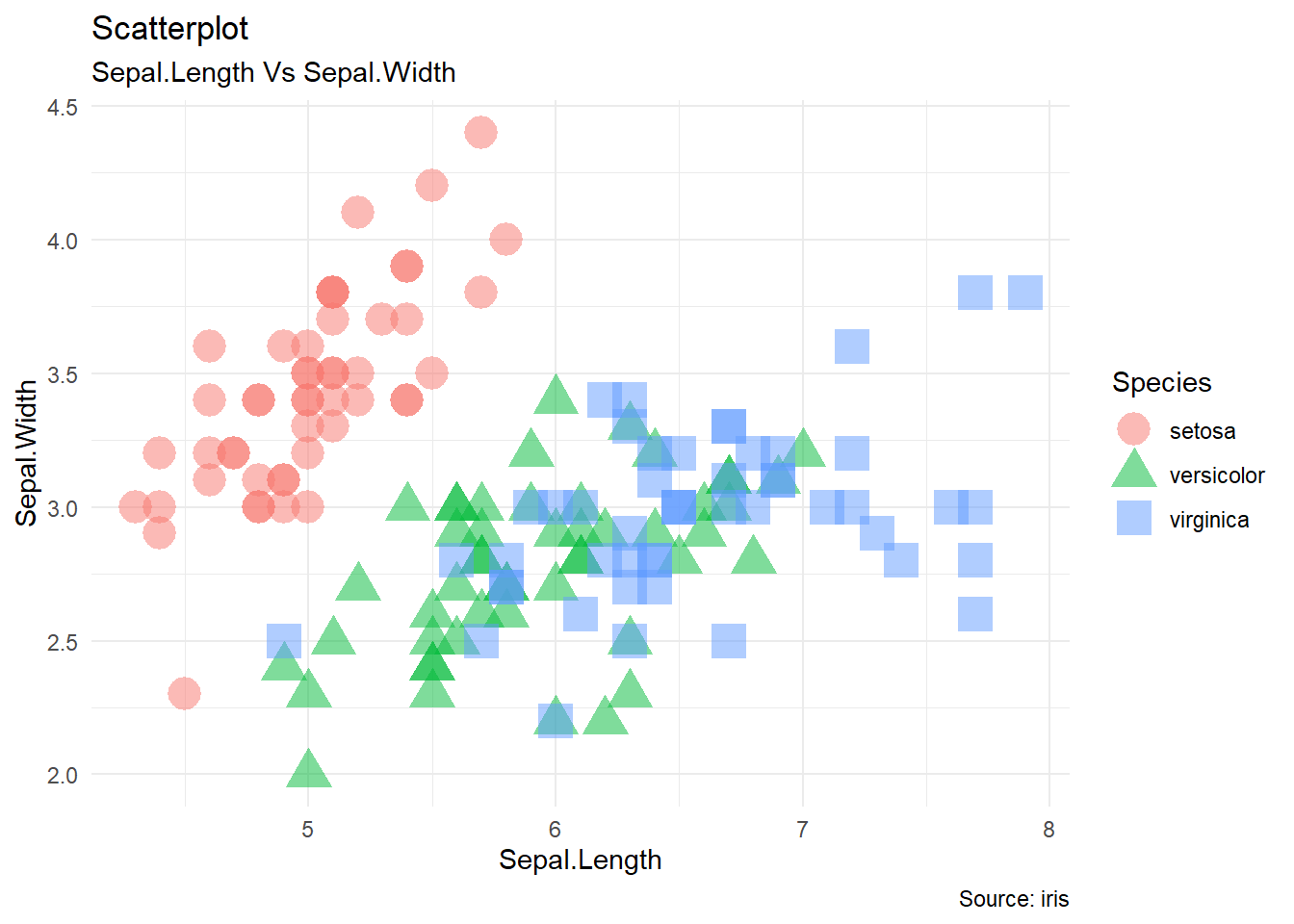
5.5 Problem 5
##   sex ageYear ageMonth heightIn weightLb
## 1   f   11.92      143     56.3     85.0
## 2   f   12.92      155     62.3    105.0
## 3   f   12.75      153     63.3    108.0
## 4   f   13.42      161     59.0     92.0
## 5   f   15.92      191     62.5    112.5
## 6 f 14.25 171 62.5 112.0ggplot(heightweight, aes(heightIn, weightLb)) +
geom_point(aes(color = sex), size = 3, alpha = 0.5) +
geom_smooth(aes(group = sex, color = sex), method = "lm", se = FALSE) +
theme_classic() +
labs(title = "Scatterplot",
subtitle = "Weight Vs Height",
caption = "Source: heightweight")## `geom_smooth()` using formula 'y ~ x'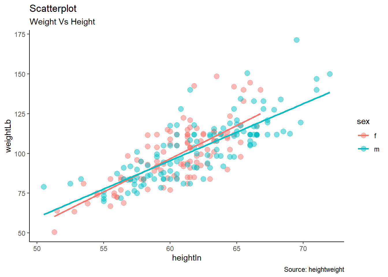
5.6 Problem 6
## # A tibble: 6 x 11
##   manufacturer model displ  year   cyl trans      drv     cty   hwy fl    class
##   <chr>        <chr> <dbl> <int> <int> <chr>      <chr> <int> <int> <chr> <chr>
## 1 audi         a4      1.8  1999     4 auto(l5)   f        18    29 p     compact
## 2 audi         a4      1.8  1999     4 manual(m5) f        21    29 p     compact
## 3 audi         a4      2    2008     4 manual(m6) f        20    31 p     compact
## 4 audi         a4      2    2008     4 auto(av)   f        21    30 p     compact
## 5 audi         a4      2.8  1999     6 auto(l5)   f        16    26 p     compact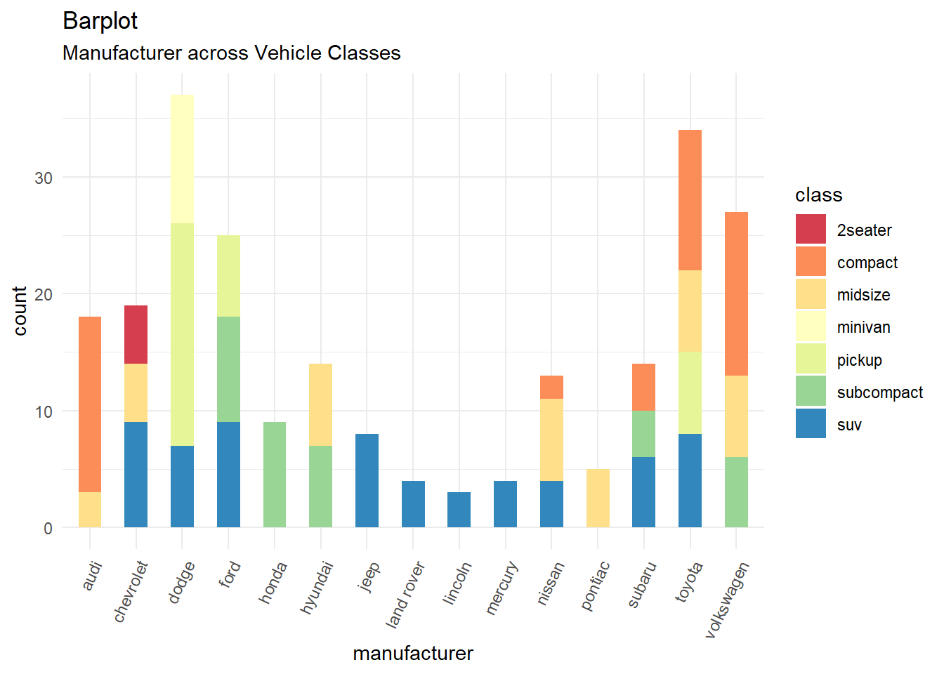
## 6 audi a4 2.8 1999 6 manual(m5) f 18 26 p compactggplot(mpg, aes(manufacturer, fill = class)) + geom_bar(width = 0.5) +
theme_minimal() +
theme(axis.text.x = element_text(angle = 65)) +
scale_fill_brewer(palette = "Spectral") +
labs(title = "Barplot",
subtitle = "Manufacturer across Vehicle Classes")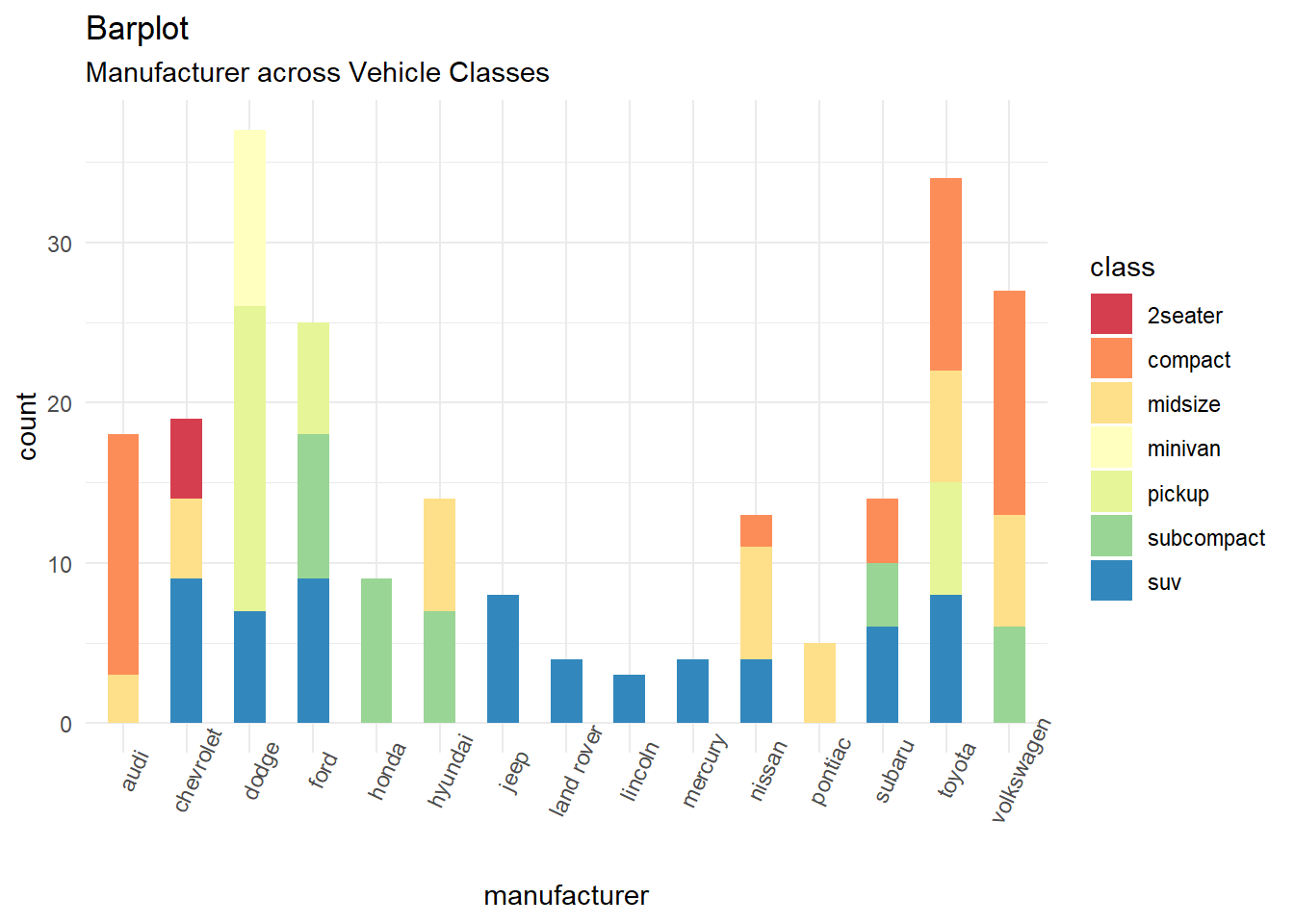
ggplot(mpg, aes(manufacturer, fill = class)) + geom_bar(width = 0.5) +
  theme_minimal() +
  theme(axis.text.x = element_text(angle = 65, hjust = 1.0)) +
  scale_fill_brewer(palette = "Spectral") +
  labs(title = "Barplot",
       subtitle = "Manufacturer across Vehicle Classes")