Chapter 8 dyplyr
10월 15일 목요일, 202AIE17 송채은
What is dplyr?
dplyr is a grammar of data manipulation, he dplyr package provides a set of functions to transform or manipulate your data into the right form you need
- verb(a data frame, what to do with the data frame)
- filter() : picks cases based on their values
- select() : picks variables based on their names
- mutate() : adds new variables that are functions of existing variables
- arrange() : changes the ordering of the rows
- summarize() : reduces multiple values down to a single summary
These all combine naturally with group_by() which allows you to perform any operation “by group”
8.1 Tibbles
we often use a data frame to store our data. A tibble is the tidyverse version of the data frame in Base R
as_tibble() : convert a data frame to a tibble
## # A tibble: 150 x 5
##    Sepal.Length Sepal.Width Petal.Length Petal.Width Species
##           <dbl>       <dbl>        <dbl>       <dbl> <fct>
##  1          5.1         3.5          1.4         0.2 setosa
##  2          4.9         3            1.4         0.2 setosa
##  3          4.7         3.2          1.3         0.2 setosa
##  4          4.6         3.1          1.5         0.2 setosa
##  5          5           3.6          1.4         0.2 setosa
##  6          5.4         3.9          1.7         0.4 setosa
##  7          4.6         3.4          1.4         0.3 setosa
##  8          5           3.4          1.5         0.2 setosa
##  9          4.4         2.9          1.4         0.2 setosa
## 10          4.9         3.1          1.5         0.1 setosa
## # ... with 140 more rows
8.2 Select columns with select()
select() subsets columns
## # A tibble: 336,776 x 19
##     year month   day dep_time sched_dep_time dep_delay arr_time sched_arr_time arr_delay carrier flight tailnum origin dest
##    <int> <int> <int>    <int>          <int>     <dbl>    <int>          <int>     <dbl> <chr>    <int> <chr>   <chr>  <chr>
##  1  2013     1     1      517            515         2      830            819        11 UA        1545 N14228  EWR    IAH
##  2  2013     1     1      533            529         4      850            830        20 UA        1714 N24211  LGA    IAH
##  3  2013     1     1      542            540         2      923            850        33 AA        1141 N619AA  JFK    MIA
##  4  2013     1     1      544            545        -1     1004           1022       -18 B6         725 N804JB  JFK    BQN
##  5  2013     1     1      554            600        -6      812            837       -25 DL         461 N668DN  LGA    ATL
##  6  2013     1     1      554            558        -4      740            728        12 UA        1696 N39463  EWR    ORD
##  7  2013     1     1      555            600        -5      913            854        19 B6         507 N516JB  EWR    FLL
##  8  2013     1     1      557            600        -3      709            723       -14 EV        5708 N829AS  LGA    IAD
##  9  2013     1     1      557            600        -3      838            846        -8 B6          79 N593JB  JFK    MCO
## 10  2013     1     1      558            600        -2      753            745         8 AA         301 N3ALAA  LGA    ORD
## # ... with 336,766 more rows, and 5 more variables: air_time <dbl>, distance <dbl>, hour <dbl>, minute <dbl>, time_hour <dttm>
names() displays column names
##  [1] "year"           "month"          "day"            "dep_time"       "sched_dep_time" "dep_delay"      "arr_time"
##  [8] "sched_arr_time" "arr_delay"      "carrier"        "flight"         "tailnum"        "origin"         "dest"
## [15] "air_time" "distance" "hour" "minute" "time_hour"## # A tibble: 336,776 x 3
## year month day
## <int> <int> <int>
## 1 2013 1 1
## 2 2013 1 1
## 3 2013 1 1
## 4 2013 1 1
## 5 2013 1 1
## 6 2013 1 1
## 7 2013 1 1
## 8 2013 1 1
## 9 2013 1 1
## 10 2013 1 1
## # ... with 336,766 more rows: for selecting a range of consecutive variables
## # A tibble: 336,776 x 3
##     year month   day
##    <int> <int> <int>
##  1  2013     1     1
##  2  2013     1     1
##  3  2013     1     1
##  4  2013     1     1
##  5  2013     1     1
##  6  2013     1     1
##  7  2013     1     1
##  8  2013     1     1
##  9  2013     1     1
## 10  2013     1     1
## # ... with 336,766 more rows! for taking the complement of a set of variables
## # A tibble: 336,776 x 16
##    dep_time sched_dep_time dep_delay arr_time sched_arr_time arr_delay carrier flight tailnum origin dest  air_time distance  hour
##       <int>          <int>     <dbl>    <int>          <int>     <dbl> <chr>    <int> <chr>   <chr>  <chr>    <dbl>    <dbl> <dbl>
##  1      517            515         2      830            819        11 UA        1545 N14228  EWR    IAH        227     1400     5
##  2      533            529         4      850            830        20 UA        1714 N24211  LGA    IAH        227     1416     5
##  3      542            540         2      923            850        33 AA        1141 N619AA  JFK    MIA        160     1089     5
##  4      544            545        -1     1004           1022       -18 B6         725 N804JB  JFK    BQN        183     1576     5
##  5      554            600        -6      812            837       -25 DL         461 N668DN  LGA    ATL        116      762     6
##  6      554            558        -4      740            728        12 UA        1696 N39463  EWR    ORD        150      719     5
##  7      555            600        -5      913            854        19 B6         507 N516JB  EWR    FLL        158     1065     6
##  8      557            600        -3      709            723       -14 EV        5708 N829AS  LGA    IAD         53      229     6
##  9      557            600        -3      838            846        -8 B6          79 N593JB  JFK    MCO        140      944     6
## 10      558            600        -2      753            745         8 AA         301 N3ALAA  LGA    ORD        138      733     6
## # ... with 336,766 more rows, and 2 more variables: minute <dbl>, time_hour <dttm>- Selection helper functions
- starts_with() : Starts with a prefix
- ends_with() : Ends with a suffix
- contains() : Contains a literal string
- matches() : Matches a regular expression
- num_range() : Matches a numerical range like x01, x02, x03
select all columns starts with “dep”
## # A tibble: 336,776 x 2
##    dep_time dep_delay
##       <int>     <dbl>
##  1      517         2
##  2      533         4
##  3      542         2
##  4      544        -1
##  5      554        -6
##  6      554        -4
##  7      555        -5
##  8      557        -3
##  9      557        -3
## 10      558        -2
## # ... with 336,766 more rows
select all columns ends with “time”
## # A tibble: 336,776 x 5
##    dep_time sched_dep_time arr_time sched_arr_time air_time
##       <int>          <int>    <int>          <int>    <dbl>
##  1      517            515      830            819      227
##  2      533            529      850            830      227
##  3      542            540      923            850      160
##  4      544            545     1004           1022      183
##  5      554            600      812            837      116
##  6      554            558      740            728      150
##  7      555            600      913            854      158
##  8      557            600      709            723       53
##  9      557            600      838            846      140
## 10      558            600      753            745      138
## # ... with 336,766 more rows
select all columns contains “time”
## # A tibble: 336,776 x 6
##    dep_time sched_dep_time arr_time sched_arr_time air_time time_hour
##       <int>          <int>    <int>          <int>    <dbl> <dttm>
##  1      517            515      830            819      227 2013-01-01 05:00:00
##  2      533            529      850            830      227 2013-01-01 05:00:00
##  3      542            540      923            850      160 2013-01-01 05:00:00
##  4      544            545     1004           1022      183 2013-01-01 05:00:00
##  5      554            600      812            837      116 2013-01-01 06:00:00
##  6      554            558      740            728      150 2013-01-01 05:00:00
##  7      555            600      913            854      158 2013-01-01 06:00:00
##  8      557            600      709            723       53 2013-01-01 06:00:00
##  9      557            600      838            846      140 2013-01-01 06:00:00
## 10      558            600      753            745      138 2013-01-01 06:00:00
## # ... with 336,766 more rows
select all columns starts with “dep”, contains “time”, and between year and day (inclusive)
## # A tibble: 336,776 x 10
##    dep_time dep_delay sched_dep_time arr_time sched_arr_time air_time time_hour            year month   day
##       <int>     <dbl>          <int>    <int>          <int>    <dbl> <dttm>              <int> <int> <int>
##  1      517         2            515      830            819      227 2013-01-01 05:00:00  2013     1     1
##  2      533         4            529      850            830      227 2013-01-01 05:00:00  2013     1     1
##  3      542         2            540      923            850      160 2013-01-01 05:00:00  2013     1     1
##  4      544        -1            545     1004           1022      183 2013-01-01 05:00:00  2013     1     1
##  5      554        -6            600      812            837      116 2013-01-01 06:00:00  2013     1     1
##  6      554        -4            558      740            728      150 2013-01-01 05:00:00  2013     1     1
##  7      555        -5            600      913            854      158 2013-01-01 06:00:00  2013     1     1
##  8      557        -3            600      709            723       53 2013-01-01 06:00:00  2013     1     1
##  9      557        -3            600      838            846      140 2013-01-01 06:00:00  2013     1     1
## 10      558        -2            600      753            745      138 2013-01-01 06:00:00  2013     1     1
## # ... with 336,766 more rows
select columns 1,3,5
## # A tibble: 336,776 x 3
##     year   day sched_dep_time
##    <int> <int>          <int>
##  1  2013     1            515
##  2  2013     1            529
##  3  2013     1            540
##  4  2013     1            545
##  5  2013     1            600
##  6  2013     1            558
##  7  2013     1            600
##  8  2013     1            600
##  9  2013     1            600
## 10  2013     1            600
## # ... with 336,766 more rows## # A tibble: 317 x 79
## artist track date.entered wk1 wk2 wk3 wk4 wk5 wk6 wk7 wk8 wk9 wk10 wk11 wk12 wk13 wk14 wk15 wk16 wk17
## <chr> <chr> <date> <dbl> <dbl> <dbl> <dbl> <dbl> <dbl> <dbl> <dbl> <dbl> <dbl> <dbl> <dbl> <dbl> <dbl> <dbl> <dbl> <dbl>
## 1 2 Pac Baby~ 2000-02-26 87 82 72 77 87 94 99 NA NA NA NA NA NA NA NA NA NA
## 2 2Ge+h~ The ~ 2000-09-02 91 87 92 NA NA NA NA NA NA NA NA NA NA NA NA NA NA
## 3 3 Doo~ Kryp~ 2000-04-08 81 70 68 67 66 57 54 53 51 51 51 51 47 44 38 28 22
## 4 3 Doo~ Loser 2000-10-21 76 76 72 69 67 65 55 59 62 61 61 59 61 66 72 76 75
## 5 504 B~ Wobb~ 2000-04-15 57 34 25 17 17 31 36 49 53 57 64 70 75 76 78 85 92
## 6 98^0 Give~ 2000-08-19 51 39 34 26 26 19 2 2 3 6 7 22 29 36 47 67 66
## 7 A*Tee~ Danc~ 2000-07-08 97 97 96 95 100 NA NA NA NA NA NA NA NA NA NA NA NA
## 8 Aaliy~ I Do~ 2000-01-29 84 62 51 41 38 35 35 38 38 36 37 37 38 49 61 63 62
## 9 Aaliy~ Try ~ 2000-03-18 59 53 38 28 21 18 16 14 12 10 9 8 6 1 2 2 2
## 10 Adams~ Open~ 2000-08-26 76 76 74 69 68 67 61 58 57 59 66 68 61 67 59 63 67
## # ... with 307 more rows, and 59 more variables: wk18 <dbl>, wk19 <dbl>, wk20 <dbl>, wk21 <dbl>, wk22 <dbl>, wk23 <dbl>,
## # wk24 <dbl>, wk25 <dbl>, wk26 <dbl>, wk27 <dbl>, wk28 <dbl>, wk29 <dbl>, wk30 <dbl>, wk31 <dbl>, wk32 <dbl>, wk33 <dbl>,
## # wk34 <dbl>, wk35 <dbl>, wk36 <dbl>, wk37 <dbl>, wk38 <dbl>, wk39 <dbl>, wk40 <dbl>, wk41 <dbl>, wk42 <dbl>, wk43 <dbl>,
## # wk44 <dbl>, wk45 <dbl>, wk46 <dbl>, wk47 <dbl>, wk48 <dbl>, wk49 <dbl>, wk50 <dbl>, wk51 <dbl>, wk52 <dbl>, wk53 <dbl>,
## # wk54 <dbl>, wk55 <dbl>, wk56 <dbl>, wk57 <dbl>, wk58 <dbl>, wk59 <dbl>, wk60 <dbl>, wk61 <dbl>, wk62 <dbl>, wk63 <dbl>,
## # wk64 <dbl>, wk65 <dbl>, wk66 <lgl>, wk67 <lgl>, wk68 <lgl>, wk69 <lgl>, wk70 <lgl>, wk71 <lgl>, wk72 <lgl>, wk73 <lgl>,
## # wk74 <lgl>, wk75 <lgl>, wk76 <lgl>names() returns columns of a dataset
##  [1] "artist"       "track"        "date.entered" "wk1"          "wk2"          "wk3"          "wk4"          "wk5"
##  [9] "wk6"          "wk7"          "wk8"          "wk9"          "wk10"         "wk11"         "wk12"         "wk13"
## [17] "wk14"         "wk15"         "wk16"         "wk17"         "wk18"         "wk19"         "wk20"         "wk21"
## [25] "wk22"         "wk23"         "wk24"         "wk25"         "wk26"         "wk27"         "wk28"         "wk29"
## [33] "wk30"         "wk31"         "wk32"         "wk33"         "wk34"         "wk35"         "wk36"         "wk37"
## [41] "wk38"         "wk39"         "wk40"         "wk41"         "wk42"         "wk43"         "wk44"         "wk45"
## [49] "wk46"         "wk47"         "wk48"         "wk49"         "wk50"         "wk51"         "wk52"         "wk53"
## [57] "wk54"         "wk55"         "wk56"         "wk57"         "wk58"         "wk59"         "wk60"         "wk61"
## [65] "wk62"         "wk63"         "wk64"         "wk65"         "wk66"         "wk67"         "wk68"         "wk69"
## [73] "wk70" "wk71" "wk72" "wk73" "wk74" "wk75" "wk76"## # A tibble: 317 x 4
## wk20 wk21 wk22 wk23
## <dbl> <dbl> <dbl> <dbl>
## 1 NA NA NA NA
## 2 NA NA NA NA
## 3 14 12 7 6
## 4 70 NA NA NA
## 5 NA NA NA NA
## 6 94 NA NA NA
## 7 NA NA NA NA
## 8 86 NA NA NA
## 9 4 5 5 6
## 10 89 NA NA NA
## # ... with 307 more rows8.3 Filter rows with filter()
filter() subsets observations based on their values
filter the flights departed on Jan 1
## # A tibble: 842 x 19
##     year month   day dep_time sched_dep_time dep_delay arr_time sched_arr_time arr_delay carrier flight tailnum origin dest
##    <int> <int> <int>    <int>          <int>     <dbl>    <int>          <int>     <dbl> <chr>    <int> <chr>   <chr>  <chr>
##  1  2013     1     1      517            515         2      830            819        11 UA        1545 N14228  EWR    IAH
##  2  2013     1     1      533            529         4      850            830        20 UA        1714 N24211  LGA    IAH
##  3  2013     1     1      542            540         2      923            850        33 AA        1141 N619AA  JFK    MIA
##  4  2013     1     1      544            545        -1     1004           1022       -18 B6         725 N804JB  JFK    BQN
##  5  2013     1     1      554            600        -6      812            837       -25 DL         461 N668DN  LGA    ATL
##  6  2013     1     1      554            558        -4      740            728        12 UA        1696 N39463  EWR    ORD
##  7  2013     1     1      555            600        -5      913            854        19 B6         507 N516JB  EWR    FLL
##  8  2013     1     1      557            600        -3      709            723       -14 EV        5708 N829AS  LGA    IAD
##  9  2013     1     1      557            600        -3      838            846        -8 B6          79 N593JB  JFK    MCO
## 10  2013     1     1      558            600        -2      753            745         8 AA         301 N3ALAA  LGA    ORD
## # ... with 832 more rows, and 5 more variables: air_time <dbl>, distance <dbl>, hour <dbl>, minute <dbl>, time_hour <dttm>
filter the flights departed on Nov or Dec
## # A tibble: 55,403 x 19
##     year month   day dep_time sched_dep_time dep_delay arr_time sched_arr_time arr_delay carrier flight tailnum origin dest
##    <int> <int> <int>    <int>          <int>     <dbl>    <int>          <int>     <dbl> <chr>    <int> <chr>   <chr>  <chr>
##  1  2013    11     1        5           2359         6      352            345         7 B6         745 N568JB  JFK    PSE
##  2  2013    11     1       35           2250       105      123           2356        87 B6        1816 N353JB  JFK    SYR
##  3  2013    11     1      455            500        -5      641            651       -10 US        1895 N192UW  EWR    CLT
##  4  2013    11     1      539            545        -6      856            827        29 UA        1714 N38727  LGA    IAH
##  5  2013    11     1      542            545        -3      831            855       -24 AA        2243 N5CLAA  JFK    MIA
##  6  2013    11     1      549            600       -11      912            923       -11 UA         303 N595UA  JFK    SFO
##  7  2013    11     1      550            600       -10      705            659         6 US        2167 N748UW  LGA    DCA
##  8  2013    11     1      554            600        -6      659            701        -2 US        2134 N742PS  LGA    BOS
##  9  2013    11     1      554            600        -6      826            827        -1 DL         563 N912DE  LGA    ATL
## 10  2013    11     1      554            600        -6      749            751        -2 DL         731 N315NB  LGA    DTW
## # ... with 55,393 more rows, and 5 more variables: air_time <dbl>, distance <dbl>, hour <dbl>, minute <dbl>, time_hour <dttm>
filter the flights to IAH
## # A tibble: 7,198 x 19
##     year month   day dep_time sched_dep_time dep_delay arr_time sched_arr_time arr_delay carrier flight tailnum origin dest
##    <int> <int> <int>    <int>          <int>     <dbl>    <int>          <int>     <dbl> <chr>    <int> <chr>   <chr>  <chr>
##  1  2013     1     1      517            515         2      830            819        11 UA        1545 N14228  EWR    IAH
##  2  2013     1     1      533            529         4      850            830        20 UA        1714 N24211  LGA    IAH
##  3  2013     1     1      623            627        -4      933            932         1 UA         496 N459UA  LGA    IAH
##  4  2013     1     1      728            732        -4     1041           1038         3 UA         473 N488UA  LGA    IAH
##  5  2013     1     1      739            739         0     1104           1038        26 UA        1479 N37408  EWR    IAH
##  6  2013     1     1      908            908         0     1228           1219         9 UA        1220 N12216  EWR    IAH
##  7  2013     1     1     1028           1026         2     1350           1339        11 UA        1004 N76508  LGA    IAH
##  8  2013     1     1     1044           1045        -1     1352           1351         1 UA         455 N667UA  EWR    IAH
##  9  2013     1     1     1114            900       134     1447           1222       145 UA        1086 N76502  LGA    IAH
## 10  2013     1     1     1205           1200         5     1503           1505        -2 UA        1461 N39418  EWR    IAH
## # ... with 7,188 more rows, and 5 more variables: air_time <dbl>, distance <dbl>, hour <dbl>, minute <dbl>, time_hour <dttm>
filter the flights with arr_delay <= 120 or dep_delay > 120
## # A tibble: 325,773 x 19
##     year month   day dep_time sched_dep_time dep_delay arr_time sched_arr_time arr_delay carrier flight tailnum origin dest
##    <int> <int> <int>    <int>          <int>     <dbl>    <int>          <int>     <dbl> <chr>    <int> <chr>   <chr>  <chr>
##  1  2013     1     1      517            515         2      830            819        11 UA        1545 N14228  EWR    IAH
##  2  2013     1     1      533            529         4      850            830        20 UA        1714 N24211  LGA    IAH
##  3  2013     1     1      542            540         2      923            850        33 AA        1141 N619AA  JFK    MIA
##  4  2013     1     1      544            545        -1     1004           1022       -18 B6         725 N804JB  JFK    BQN
##  5  2013     1     1      554            600        -6      812            837       -25 DL         461 N668DN  LGA    ATL
##  6  2013     1     1      554            558        -4      740            728        12 UA        1696 N39463  EWR    ORD
##  7  2013     1     1      555            600        -5      913            854        19 B6         507 N516JB  EWR    FLL
##  8  2013     1     1      557            600        -3      709            723       -14 EV        5708 N829AS  LGA    IAD
##  9  2013     1     1      557            600        -3      838            846        -8 B6          79 N593JB  JFK    MCO
## 10  2013     1     1      558            600        -2      753            745         8 AA         301 N3ALAA  LGA    ORD
## # ... with 325,763 more rows, and 5 more variables: air_time <dbl>, distance <dbl>, hour <dbl>, minute <dbl>, time_hour <dttm>
8.4 Add new variables with mutate()
mutate() create a new variable
mutate() executes the transformations iteratively so that later transformations can use the columns created by earlier transformations
## # A tibble: 336,776 x 22
##     year month   day dep_time sched_dep_time dep_delay arr_time sched_arr_time arr_delay carrier flight tailnum origin dest
##    <int> <int> <int>    <int>          <int>     <dbl>    <int>          <int>     <dbl> <chr>    <int> <chr>   <chr>  <chr>
##  1  2013     1     1      517            515         2      830            819        11 UA        1545 N14228  EWR    IAH
##  2  2013     1     1      533            529         4      850            830        20 UA        1714 N24211  LGA    IAH
##  3  2013     1     1      542            540         2      923            850        33 AA        1141 N619AA  JFK    MIA
##  4  2013     1     1      544            545        -1     1004           1022       -18 B6         725 N804JB  JFK    BQN
##  5  2013     1     1      554            600        -6      812            837       -25 DL         461 N668DN  LGA    ATL
##  6  2013     1     1      554            558        -4      740            728        12 UA        1696 N39463  EWR    ORD
##  7  2013     1     1      555            600        -5      913            854        19 B6         507 N516JB  EWR    FLL
##  8  2013     1     1      557            600        -3      709            723       -14 EV        5708 N829AS  LGA    IAD
##  9  2013     1     1      557            600        -3      838            846        -8 B6          79 N593JB  JFK    MCO
## 10  2013     1     1      558            600        -2      753            745         8 AA         301 N3ALAA  LGA    ORD
## # ... with 336,766 more rows, and 8 more variables: air_time <dbl>, distance <dbl>, hour <dbl>, minute <dbl>, time_hour <dttm>,
## #   gain <dbl>, hours <dbl>, gain_per_hour <dbl>
transmute() creates a new variable but drops others
transmute(flights, gain = arr_delay - dep_delay, hours = air_time / 60, gain_per_hour = gain / hours)## # A tibble: 336,776 x 3
## gain hours gain_per_hour
## <dbl> <dbl> <dbl>
## 1 9 3.78 2.38
## 2 16 3.78 4.23
## 3 31 2.67 11.6
## 4 -17 3.05 -5.57
## 5 -19 1.93 -9.83
## 6 16 2.5 6.4
## 7 24 2.63 9.11
## 8 -11 0.883 -12.5
## 9 -5 2.33 -2.14
## 10 10 2.3 4.35
## # ... with 336,766 more rowsThe scoped variant of mutate() and transmute() help us to apply the same transformation to multiple variables - mutate_all() and transmute_all() affect every variable - mutate_at() and transmute_at() affect variables selected with a character vector - mutate_if() and transmute_if() affect variables selected with a predicate function (a function that returns TRUE or FALSE)
## Sepal.Length Sepal.Width Petal.Length Petal.Width Species
## 1 5.1 3.5 1.4 0.2 setosa
## 2 4.9 3.0 1.4 0.2 setosa
## 3 4.7 3.2 1.3 0.2 setosa
## 4 4.6 3.1 1.5 0.2 setosa
## 5 5.0 3.6 1.4 0.2 setosa
## 6 5.4 3.9 1.7 0.4 setosa
## 7 4.6 3.4 1.4 0.3 setosa
## 8 5.0 3.4 1.5 0.2 setosa
## 9 4.4 2.9 1.4 0.2 setosa
## 10 4.9 3.1 1.5 0.1 setosa
## 11 5.4 3.7 1.5 0.2 setosa
## 12 4.8 3.4 1.6 0.2 setosa
## 13 4.8 3.0 1.4 0.1 setosa
## 14 4.3 3.0 1.1 0.1 setosa
## 15 5.8 4.0 1.2 0.2 setosa
## 16 5.7 4.4 1.5 0.4 setosa
## 17 5.4 3.9 1.3 0.4 setosa
## 18 5.1 3.5 1.4 0.3 setosa
## 19 5.7 3.8 1.7 0.3 setosa
## 20 5.1 3.8 1.5 0.3 setosa
## 21 5.4 3.4 1.7 0.2 setosa
## 22 5.1 3.7 1.5 0.4 setosa
## 23 4.6 3.6 1.0 0.2 setosa
## 24 5.1 3.3 1.7 0.5 setosa
## 25 4.8 3.4 1.9 0.2 setosa
## 26 5.0 3.0 1.6 0.2 setosa
## 27 5.0 3.4 1.6 0.4 setosa
## 28 5.2 3.5 1.5 0.2 setosa
## 29 5.2 3.4 1.4 0.2 setosa
## 30 4.7 3.2 1.6 0.2 setosa
## 31 4.8 3.1 1.6 0.2 setosa
## 32 5.4 3.4 1.5 0.4 setosa
## 33 5.2 4.1 1.5 0.1 setosa
## 34 5.5 4.2 1.4 0.2 setosa
## 35 4.9 3.1 1.5 0.2 setosa
## 36 5.0 3.2 1.2 0.2 setosa
## 37 5.5 3.5 1.3 0.2 setosa
## 38 4.9 3.6 1.4 0.1 setosa
## 39 4.4 3.0 1.3 0.2 setosa
## 40 5.1 3.4 1.5 0.2 setosa
## 41 5.0 3.5 1.3 0.3 setosa
## 42 4.5 2.3 1.3 0.3 setosa
## 43 4.4 3.2 1.3 0.2 setosa
## 44 5.0 3.5 1.6 0.6 setosa
## 45 5.1 3.8 1.9 0.4 setosa
## 46 4.8 3.0 1.4 0.3 setosa
## 47 5.1 3.8 1.6 0.2 setosa
## 48 4.6 3.2 1.4 0.2 setosa
## 49 5.3 3.7 1.5 0.2 setosa
## 50 5.0 3.3 1.4 0.2 setosa
## 51 7.0 3.2 4.7 1.4 versicolor
## 52 6.4 3.2 4.5 1.5 versicolor
## 53 6.9 3.1 4.9 1.5 versicolor
## 54 5.5 2.3 4.0 1.3 versicolor
## 55 6.5 2.8 4.6 1.5 versicolor
## 56 5.7 2.8 4.5 1.3 versicolor
## 57 6.3 3.3 4.7 1.6 versicolor
## 58 4.9 2.4 3.3 1.0 versicolor
## 59 6.6 2.9 4.6 1.3 versicolor
## 60 5.2 2.7 3.9 1.4 versicolor
## 61 5.0 2.0 3.5 1.0 versicolor
## 62 5.9 3.0 4.2 1.5 versicolor
## 63 6.0 2.2 4.0 1.0 versicolor
## 64 6.1 2.9 4.7 1.4 versicolor
## 65 5.6 2.9 3.6 1.3 versicolor
## 66 6.7 3.1 4.4 1.4 versicolor
## 67 5.6 3.0 4.5 1.5 versicolor
## 68 5.8 2.7 4.1 1.0 versicolor
## 69 6.2 2.2 4.5 1.5 versicolor
## 70 5.6 2.5 3.9 1.1 versicolor
## 71 5.9 3.2 4.8 1.8 versicolor
## 72 6.1 2.8 4.0 1.3 versicolor
## 73 6.3 2.5 4.9 1.5 versicolor
## 74 6.1 2.8 4.7 1.2 versicolor
## 75 6.4 2.9 4.3 1.3 versicolor
## 76 6.6 3.0 4.4 1.4 versicolor
## 77 6.8 2.8 4.8 1.4 versicolor
## 78 6.7 3.0 5.0 1.7 versicolor
## 79 6.0 2.9 4.5 1.5 versicolor
## 80 5.7 2.6 3.5 1.0 versicolor
## 81 5.5 2.4 3.8 1.1 versicolor
## 82 5.5 2.4 3.7 1.0 versicolor
## 83 5.8 2.7 3.9 1.2 versicolor
## 84 6.0 2.7 5.1 1.6 versicolor
## 85 5.4 3.0 4.5 1.5 versicolor
## 86 6.0 3.4 4.5 1.6 versicolor
## 87 6.7 3.1 4.7 1.5 versicolor
## 88 6.3 2.3 4.4 1.3 versicolor
## 89 5.6 3.0 4.1 1.3 versicolor
## 90 5.5 2.5 4.0 1.3 versicolor
## 91 5.5 2.6 4.4 1.2 versicolor
## 92 6.1 3.0 4.6 1.4 versicolor
## 93 5.8 2.6 4.0 1.2 versicolor
## 94 5.0 2.3 3.3 1.0 versicolor
## 95 5.6 2.7 4.2 1.3 versicolor
## 96 5.7 3.0 4.2 1.2 versicolor
## 97 5.7 2.9 4.2 1.3 versicolor
## 98 6.2 2.9 4.3 1.3 versicolor
## 99 5.1 2.5 3.0 1.1 versicolor
## 100 5.7 2.8 4.1 1.3 versicolor
## 101 6.3 3.3 6.0 2.5 virginica
## 102 5.8 2.7 5.1 1.9 virginica
## 103 7.1 3.0 5.9 2.1 virginica
## 104 6.3 2.9 5.6 1.8 virginica
## 105 6.5 3.0 5.8 2.2 virginica
## 106 7.6 3.0 6.6 2.1 virginica
## 107 4.9 2.5 4.5 1.7 virginica
## 108 7.3 2.9 6.3 1.8 virginica
## 109 6.7 2.5 5.8 1.8 virginica
## 110 7.2 3.6 6.1 2.5 virginica
## 111 6.5 3.2 5.1 2.0 virginica
## 112 6.4 2.7 5.3 1.9 virginica
## 113 6.8 3.0 5.5 2.1 virginica
## 114 5.7 2.5 5.0 2.0 virginica
## 115 5.8 2.8 5.1 2.4 virginica
## 116 6.4 3.2 5.3 2.3 virginica
## 117 6.5 3.0 5.5 1.8 virginica
## 118 7.7 3.8 6.7 2.2 virginica
## 119 7.7 2.6 6.9 2.3 virginica
## 120 6.0 2.2 5.0 1.5 virginica
## 121 6.9 3.2 5.7 2.3 virginica
## 122 5.6 2.8 4.9 2.0 virginica
## 123 7.7 2.8 6.7 2.0 virginica
## 124 6.3 2.7 4.9 1.8 virginica
## 125 6.7 3.3 5.7 2.1 virginica
## 126 7.2 3.2 6.0 1.8 virginica
## 127 6.2 2.8 4.8 1.8 virginica
## 128 6.1 3.0 4.9 1.8 virginica
## 129 6.4 2.8 5.6 2.1 virginica
## 130 7.2 3.0 5.8 1.6 virginica
## 131 7.4 2.8 6.1 1.9 virginica
## 132 7.9 3.8 6.4 2.0 virginica
## 133 6.4 2.8 5.6 2.2 virginica
## 134 6.3 2.8 5.1 1.5 virginica
## 135 6.1 2.6 5.6 1.4 virginica
## 136 7.7 3.0 6.1 2.3 virginica
## 137 6.3 3.4 5.6 2.4 virginica
## 138 6.4 3.1 5.5 1.8 virginica
## 139 6.0 3.0 4.8 1.8 virginica
## 140 6.9 3.1 5.4 2.1 virginica
## 141 6.7 3.1 5.6 2.4 virginica
## 142 6.9 3.1 5.1 2.3 virginica
## 143 5.8 2.7 5.1 1.9 virginica
## 144 6.8 3.2 5.9 2.3 virginica
## 145 6.7 3.3 5.7 2.5 virginica
## 146 6.7 3.0 5.2 2.3 virginica
## 147 6.3 2.5 5.0 1.9 virginica
## 148 6.5 3.0 5.2 2.0 virginica
## 149 6.2 3.4 5.4 2.3 virginica
## 150 5.9 3.0 5.1 1.8 virginicaapply log() to the columns that contain “Sepal”
##   Sepal.Length Sepal.Width Petal.Length Petal.Width Species
## 1     1.629241    1.252763          1.4         0.2  setosa
## 2     1.589235    1.098612          1.4         0.2  setosa
## 3     1.547563    1.163151          1.3         0.2  setosa
## 4     1.526056    1.131402          1.5         0.2  setosa
## 5     1.609438    1.280934          1.4         0.2  setosa
## 6     1.686399    1.360977          1.7         0.4  setosa
apply log() to the numeric columns
##   Sepal.Length Sepal.Width Petal.Length Petal.Width Species
## 1     1.629241    1.252763    0.3364722  -1.6094379  setosa
## 2     1.589235    1.098612    0.3364722  -1.6094379  setosa
## 3     1.547563    1.163151    0.2623643  -1.6094379  setosa
## 4     1.526056    1.131402    0.4054651  -1.6094379  setosa
## 5     1.609438    1.280934    0.3364722  -1.6094379  setosa
## 6     1.686399    1.360977    0.5306283  -0.9162907  setosa
8.5 Arrange rows with arrange()
arrange() reorders rows in ascending order by default (use desc() to order in descending order)
## # A tibble: 336,776 x 19
##     year month   day dep_time sched_dep_time dep_delay arr_time sched_arr_time arr_delay carrier flight tailnum origin dest
##    <int> <int> <int>    <int>          <int>     <dbl>    <int>          <int>     <dbl> <chr>    <int> <chr>   <chr>  <chr>
##  1  2013     1     1      517            515         2      830            819        11 UA        1545 N14228  EWR    IAH
##  2  2013     1     1      533            529         4      850            830        20 UA        1714 N24211  LGA    IAH
##  3  2013     1     1      542            540         2      923            850        33 AA        1141 N619AA  JFK    MIA
##  4  2013     1     1      544            545        -1     1004           1022       -18 B6         725 N804JB  JFK    BQN
##  5  2013     1     1      554            600        -6      812            837       -25 DL         461 N668DN  LGA    ATL
##  6  2013     1     1      554            558        -4      740            728        12 UA        1696 N39463  EWR    ORD
##  7  2013     1     1      555            600        -5      913            854        19 B6         507 N516JB  EWR    FLL
##  8  2013     1     1      557            600        -3      709            723       -14 EV        5708 N829AS  LGA    IAD
##  9  2013     1     1      557            600        -3      838            846        -8 B6          79 N593JB  JFK    MCO
## 10  2013     1     1      558            600        -2      753            745         8 AA         301 N3ALAA  LGA    ORD
## # ... with 336,766 more rows, and 5 more variables: air_time <dbl>, distance <dbl>, hour <dbl>, minute <dbl>, time_hour <dttm>## # A tibble: 336,776 x 19
## year month day dep_time sched_dep_time dep_delay arr_time sched_arr_time arr_delay carrier flight tailnum origin dest
## <int> <int> <int> <int> <int> <dbl> <int> <int> <dbl> <chr> <int> <chr> <chr> <chr>
## 1 2013 12 1 13 2359 14 446 445 1 B6 745 N715JB JFK PSE
## 2 2013 12 1 17 2359 18 443 437 6 B6 839 N593JB JFK BQN
## 3 2013 12 1 453 500 -7 636 651 -15 US 1895 N197UW EWR CLT
## 4 2013 12 1 520 515 5 749 808 -19 UA 1487 N69804 EWR IAH
## 5 2013 12 1 536 540 -4 845 850 -5 AA 2243 N634AA JFK MIA
## 6 2013 12 1 540 550 -10 1005 1027 -22 B6 939 N821JB JFK BQN
## 7 2013 12 1 541 545 -4 734 755 -21 EV 3819 N13968 EWR CVG
## 8 2013 12 1 546 545 1 826 835 -9 UA 1441 N23708 LGA IAH
## 9 2013 12 1 549 600 -11 648 659 -11 US 2167 N945UW LGA DCA
## 10 2013 12 1 550 600 -10 825 854 -29 B6 605 N706JB EWR FLL
## # ... with 336,766 more rows, and 5 more variables: air_time <dbl>, distance <dbl>, hour <dbl>, minute <dbl>, time_hour <dttm>8.6 Grouped summaries with summarize()
summarize() collapses a tibble to a single row for summary (imagine the sum and average function in Excel)
Summary functions takes a vector as an input and return a single value as an output : Counts, Locations, Position
summarize(flights, delay_mean = mean(dep_delay, na.rm = TRUE), delay_sd = sd(dep_delay, na.rm = TRUE))## # A tibble: 1 x 2
## delay_mean delay_sd
## <dbl> <dbl>
## 1 12.6 40.2Together __group_by()__, __summarize()__ will produce one row for each group
## # A tibble: 365 x 4
## # Groups:   year, month [12]
##     year month   day delay
##    <int> <int> <int> <dbl>
##  1  2013     1     1 11.5
##  2  2013     1     2 13.9
##  3  2013     1     3 11.0
##  4  2013     1     4  8.95
##  5  2013     1     5  5.73
##  6  2013     1     6  7.15
##  7  2013     1     7  5.42
##  8  2013     1     8  2.55
##  9  2013     1     9  2.28
## 10  2013     1    10  2.84
## # ... with 355 more rows## # A tibble: 150 x 5
## Sepal.Length Sepal.Width Petal.Length Petal.Width Species
## <dbl> <dbl> <dbl> <dbl> <fct>
## 1 5.1 3.5 1.4 0.2 setosa
## 2 4.9 3 1.4 0.2 setosa
## 3 4.7 3.2 1.3 0.2 setosa
## 4 4.6 3.1 1.5 0.2 setosa
## 5 5 3.6 1.4 0.2 setosa
## 6 5.4 3.9 1.7 0.4 setosa
## 7 4.6 3.4 1.4 0.3 setosa
## 8 5 3.4 1.5 0.2 setosa
## 9 4.4 2.9 1.4 0.2 setosa
## 10 4.9 3.1 1.5 0.1 setosa
## # ... with 140 more rowswithout the pipe operator %>%
## # A tibble: 3 x 5
##   Species    Sepal.Length Sepal.Width Petal.Length Petal.Width
##   <fct>             <dbl>       <dbl>        <dbl>       <dbl>
## 1 setosa             5.01        3.43         1.46       0.246
## 2 versicolor         5.94        2.77         4.26       1.33
## 3 virginica          6.59        2.97         5.55       2.03
with the pipe operator %>%
## # A tibble: 3 x 5
##   Species    Sepal.Length Sepal.Width Petal.Length Petal.Width
##   <fct>             <dbl>       <dbl>        <dbl>       <dbl>
## 1 setosa             5.01        3.43         1.46       0.246
## 2 versicolor         5.94        2.77         4.26       1.33
## 3 virginica 6.59 2.97 5.55 2.03## # A tibble: 3 x 3
## Species Sepal.Length Sepal.Width
## <fct> <dbl> <dbl>
## 1 setosa 5.01 3.43
## 2 versicolor 5.94 2.77
## 3 virginica 6.59 2.97data() loads specific data sets
## # A tibble: 600 x 15
##       id gender race         ses    sch     prog       locus concept   mot career     read write  math   sci    ss
##    <dbl> <fct>  <fct>        <fct>  <fct>   <fct>      <dbl>   <dbl> <dbl> <fct>     <dbl> <dbl> <dbl> <dbl> <dbl>
##  1    55 female hispanic     low    public  general  -1.78     0.560 1     prof1      28.3  46.3  42.8  44.4  50.6
##  2   114 male   african-amer middle public  academic  0.240   -0.350 1     operative  30.5  35.9  36.9  33.6  40.6
##  3   490 male   white        middle public  vocation -1.28     0.340 0.330 prof1      31    35.9  46.1  39    45.6
##  4    44 female hispanic     low    public  vocation  0.220   -0.760 1     service    31    41.1  49.2  33.6  35.6
##  5    26 female hispanic     middle public  academic  1.12    -0.740 0.670 service    31    41.1  36    36.9  45.6
##  6   510 male   white        middle public  vocation -0.860    1.19  0.330 operative  33.6  28.1  31.8  39.6  35.6
##  7   133 female african-amer low    public  vocation -0.230    0.440 0.330 school     33.6  35.2  40.9  29.3  25.7
##  8   213 female white        low    public  general   0.0400  -0.470 0.670 clerical   33.6  59.3  44.7  47.1  45.6
##  9   548 female white        middle private academic  0.470    0.340 0.670 prof2      33.6  43    41    49.8  35.6
## 10   309 female white        high   public  general   0.320    0.900 0.670 prof2      33.6  51.5  41.9  49.8  50.6
## # ... with 590 more rows
names() displays the column names of the HSB data
##  [1] "id"      "gender"  "race"    "ses"     "sch"     "prog"    "locus"   "concept" "mot"     "career"  "read"    "write"
## [13] "math" "sci" "ss"## tibble [600 x 15] (S3: tbl_df/tbl/data.frame)
## $ id : num [1:600] 55 114 490 44 26 510 133 213 548 309 ...
## $ gender : Factor w/ 2 levels "male","female": 2 1 1 2 2 1 2 2 2 2 ...
## $ race : Factor w/ 4 levels "hispanic","asian",..: 1 3 4 1 1 4 3 4 4 4 ...
## $ ses : Factor w/ 3 levels "low","middle",..: 1 2 2 1 2 2 1 1 2 3 ...
## $ sch : Factor w/ 2 levels "public","private": 1 1 1 1 1 1 1 1 2 1 ...
## $ prog : Factor w/ 3 levels "general","academic",..: 1 2 3 3 2 3 3 1 2 1 ...
## $ locus : num [1:600] -1.78 0.24 -1.28 0.22 1.12 ...
## $ concept: num [1:600] 0.56 -0.35 0.34 -0.76 -0.74 ...
## $ mot : num [1:600] 1 1 0.33 1 0.67 ...
## $ career : Factor w/ 17 levels "clerical","craftsman",..: 9 8 9 15 15 8 14 1 10 10 ...
## $ read : num [1:600] 28.3 30.5 31 31 31 ...
## $ write : num [1:600] 46.3 35.9 35.9 41.1 41.1 ...
## $ math : num [1:600] 42.8 36.9 46.1 49.2 36 ...
## $ sci : num [1:600] 44.4 33.6 39 33.6 36.9 ...
## $ ss : num [1:600] 50.6 40.6 45.6 35.6 45.6 ...n() gives the current group size
## # A tibble: 4 x 2
##   race             n
##   <fct>        <int>
## 1 hispanic        71
## 2 asian           34
## 3 african-amer    58
## 4 white          437
count() counts the unique values of variables
## # A tibble: 4 x 2
##   race             n
##   <fct>        <int>
## 1 hispanic        71
## 2 asian           34
## 3 african-amer    58
## 4 white 437## # A tibble: 8 x 3
## race gender n
## <fct> <fct> <int>
## 1 hispanic male 37
## 2 hispanic female 34
## 3 asian male 15
## 4 asian female 19
## 5 african-amer male 24
## 6 african-amer female 34
## 7 white male 197
## 8 white female 240the means of reading, writing, math, and social science scores
## # A tibble: 1 x 4
##   readm writem mathm   ssm
##   <dbl>  <dbl> <dbl> <dbl>
## 1  51.9   52.4  51.8  52.0
the means of reading, writing, math, and social science scores by gender
HSB_tbl %>%
  group_by(gender) %>%
  summarise(readm = mean(read), writem = mean(write), mathm = mean(math), ssm = mean(ss))
## # A tibble: 2 x 5
## gender readm writem mathm ssm
## <fct> <dbl> <dbl> <dbl> <dbl>
## 1 male 52.4 49.8 52.3 51.4
## 2 female 51.5 54.6 51.4 52.6the means of all numeric variables by gender
## # A tibble: 2 x 10
##   gender    id  locus concept   mot  read write  math   sci    ss
##   <fct>  <dbl>  <dbl>   <dbl> <dbl> <dbl> <dbl> <dbl> <dbl> <dbl>
## 1 male    305. 0.0134  0.102  0.624  52.4  49.8  52.3  53.2  51.4
## 2 female  297. 0.166  -0.0762 0.692  51.5  54.6  51.4  50.5  52.6
the means of all numeric variables by ses for only asian and hispanic
HSB_tbl %>%
  filter(race %in% c("asian", "hispanic")) %>%
  group_by(ses) %>%
  summarise(across(where(is.numeric), mean, na.rm = TRUE))
## # A tibble: 3 x 10
## ses id locus concept mot read write math sci ss
## <fct> <dbl> <dbl> <dbl> <dbl> <dbl> <dbl> <dbl> <dbl> <dbl>
## 1 low 44.8 -0.142 -0.189 0.537 44.7 45.9 45.8 43.0 45.5
## 2 middle 50.8 -0.122 0.0525 0.584 47.3 48.6 48.3 47.5 47.9
## 3 high 66.9 0.118 0.0619 0.705 55.6 55.9 56.6 54.0 55.08.7 The pipe operator %>%
x %>% f(y) turns into f(x, y)
x %>% f(y) %>% g(z) turns into g(f(x,y), z)
## # A tibble: 336,776 x 19
## # Groups:   dest [105]
##     year month   day dep_time sched_dep_time dep_delay arr_time sched_arr_time arr_delay carrier flight tailnum origin dest
##    <int> <int> <int>    <int>          <int>     <dbl>    <int>          <int>     <dbl> <chr>    <int> <chr>   <chr>  <chr>
##  1  2013     1     1      517            515         2      830            819        11 UA        1545 N14228  EWR    IAH
##  2  2013     1     1      533            529         4      850            830        20 UA        1714 N24211  LGA    IAH
##  3  2013     1     1      542            540         2      923            850        33 AA        1141 N619AA  JFK    MIA
##  4  2013     1     1      544            545        -1     1004           1022       -18 B6         725 N804JB  JFK    BQN
##  5  2013     1     1      554            600        -6      812            837       -25 DL         461 N668DN  LGA    ATL
##  6  2013     1     1      554            558        -4      740            728        12 UA        1696 N39463  EWR    ORD
##  7  2013     1     1      555            600        -5      913            854        19 B6         507 N516JB  EWR    FLL
##  8  2013     1     1      557            600        -3      709            723       -14 EV        5708 N829AS  LGA    IAD
##  9  2013     1     1      557            600        -3      838            846        -8 B6          79 N593JB  JFK    MCO
## 10  2013     1     1      558            600        -2      753            745         8 AA         301 N3ALAA  LGA    ORD
## # ... with 336,766 more rows, and 5 more variables: air_time <dbl>, distance <dbl>, hour <dbl>, minute <dbl>, time_hour <dttm>
delay <- summarize(by_dest, count = n(), dist = mean(distance, na.rm = TRUE), delay = mean(arr_delay, na.rm = TRUE)) ## # A tibble: 96 x 4
## dest count dist delay
## <chr> <int> <dbl> <dbl>
## 1 ABQ 254 1826 4.38
## 2 ACK 265 199 4.85
## 3 ALB 439 143 14.4
## 4 ATL 17215 757. 11.3
## 5 AUS 2439 1514. 6.02
## 6 AVL 275 584. 8.00
## 7 BDL 443 116 7.05
## 8 BGR 375 378 8.03
## 9 BHM 297 866. 16.9
## 10 BNA 6333 758. 11.8
## # ... with 86 more rowsggplot(delay, aes(x = dist, y = delay)) +
geom_point(aes(size = count), alpha = 1/3) +
geom_smooth(se = FALSE)## `geom_smooth()` using method = 'loess' and formula 'y ~ x'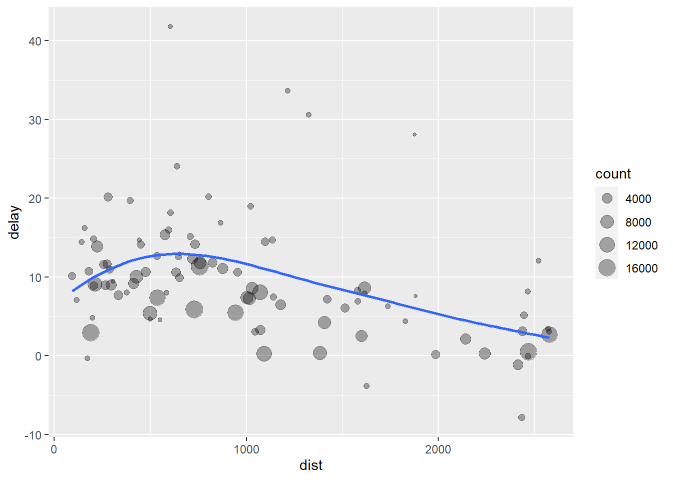
flights %>%
  group_by(dest) %>%
  summarize(count = n(), dist = mean(distance, na.rm = TRUE), delay = mean(arr_delay, na.rm = TRUE)) %>%
  filter(count > 20, dest != "HNL") %>%
  ggplot(aes(dist, delay)) +
    geom_point(aes(size = count), alpha = 1/3) +
    geom_smooth(se = FALSE)
## `geom_smooth()` using method = 'loess' and formula 'y ~ x'
8.8 Mutating joins
A join is a way of matching each row in x to zero, one, or more rows in y
The variables used to match two data frames are called key variables(or keys)
The mutating joins add columns from one data frame y to another data frame x by matching rows based the key variable
inner_join() keeps observations that appear in both data frames
left_join() keeps all observations in x
right_join() keeps all observations in y
full_join() keeps all observations in x and y
tribble() creates a tibble
## # A tibble: 3 x 2
##     key val_x
##   <dbl> <chr>
## 1     1 x1
## 2     2 x2
## 3 3 x3## # A tibble: 3 x 2
## key val_y
## <dbl> <chr>
## 1 1 y1
## 2 2 y2
## 3 4 y3inner_join() keeps observations that appear in both data frames
## # A tibble: 2 x 3
##     key val_x val_y
##   <dbl> <chr> <chr>
## 1     1 x1    y1
## 2 2 x2 y2## # A tibble: 2 x 3
## key val_x val_y
## <dbl> <chr> <chr>
## 1 1 x1 y1
## 2 2 x2 y2left_join() keeps all observations in x
## # A tibble: 3 x 3
##     key val_x val_y
##   <dbl> <chr> <chr>
## 1     1 x1    y1
## 2     2 x2    y2
## 3 3 x3 <NA>## # A tibble: 3 x 3
## key val_x val_y
## <dbl> <chr> <chr>
## 1 1 x1 y1
## 2 2 x2 y2
## 3 3 x3 <NA>right_join() keeps all observations in y
## # A tibble: 3 x 3
##     key val_x val_y
##   <dbl> <chr> <chr>
## 1     1 x1    y1
## 2     2 x2    y2
## 3 4 <NA> y3## # A tibble: 3 x 3
## key val_x val_y
## <dbl> <chr> <chr>
## 1 1 x1 y1
## 2 2 x2 y2
## 3 4 <NA> y3full_join() keeps all observations in x and y
## # A tibble: 4 x 3
##     key val_x val_y
##   <dbl> <chr> <chr>
## 1     1 x1    y1
## 2     2 x2    y2
## 3     3 x3    <NA>
## 4 4 <NA> y3## # A tibble: 4 x 3
## key val_x val_y
## <dbl> <chr> <chr>
## 1 1 x1 y1
## 2 2 x2 y2
## 3 3 x3 <NA>
## 4 4 <NA> y38.9 dyplyr practice
8.9.1 starwars data
## # A tibble: 87 x 14
##    name       height  mass hair_color   skin_color  eye_color birth_year sex   gender  homeworld species films  vehicles starships
##    <chr>       <int> <dbl> <chr>        <chr>       <chr>          <dbl> <chr> <chr>   <chr>     <chr>   <list> <list>   <list>
##  1 Luke Skyw~    172    77 blond        fair        blue            19   male  mascul~ Tatooine  Human   <chr ~ <chr [2~ <chr [2]>
##  2 C-3PO         167    75 <NA>         gold        yellow         112   none  mascul~ Tatooine  Droid   <chr ~ <chr [0~ <chr [0]>
##  3 R2-D2          96    32 <NA>         white, blue red             33   none  mascul~ Naboo     Droid   <chr ~ <chr [0~ <chr [0]>
##  4 Darth Vad~    202   136 none         white       yellow          41.9 male  mascul~ Tatooine  Human   <chr ~ <chr [0~ <chr [1]>
##  5 Leia Orga~    150    49 brown        light       brown           19   fema~ femini~ Alderaan  Human   <chr ~ <chr [1~ <chr [0]>
##  6 Owen Lars     178   120 brown, grey  light       blue            52   male  mascul~ Tatooine  Human   <chr ~ <chr [0~ <chr [0]>
##  7 Beru Whit~    165    75 brown        light       blue            47   fema~ femini~ Tatooine  Human   <chr ~ <chr [0~ <chr [0]>
##  8 R5-D4          97    32 <NA>         white, red  red             NA   none  mascul~ Tatooine  Droid   <chr ~ <chr [0~ <chr [0]>
##  9 Biggs Dar~    183    84 black        light       brown           24   male  mascul~ Tatooine  Human   <chr ~ <chr [0~ <chr [1]>
## 10 Obi-Wan K~    182    77 auburn, whi~ fair        blue-gray       57   male  mascul~ Stewjon   Human   <chr ~ <chr [1~ <chr [5]>
## # ... with 77 more rows
similar to str() in Base R
## Rows: 87
## Columns: 14
## $ name       <chr> "Luke Skywalker", "C-3PO", "R2-D2", "Darth Vader", "Leia Organa", "Owen Lars", "Beru Whitesun lars", "R5-D...
## $ height     <int> 172, 167, 96, 202, 150, 178, 165, 97, 183, 182, 188, 180, 228, 180, 173, 175, 170, 180, 66, 170, 183, 200,...
## $ mass       <dbl> 77.0, 75.0, 32.0, 136.0, 49.0, 120.0, 75.0, 32.0, 84.0, 77.0, 84.0, NA, 112.0, 80.0, 74.0, 1358.0, 77.0, 1...
## $ hair_color <chr> "blond", NA, NA, "none", "brown", "brown, grey", "brown", NA, "black", "auburn, white", "blond", "auburn, ...
## $ skin_color <chr> "fair", "gold", "white, blue", "white", "light", "light", "light", "white, red", "light", "fair", "fair", ...
## $ eye_color  <chr> "blue", "yellow", "red", "yellow", "brown", "blue", "blue", "red", "brown", "blue-gray", "blue", "blue", "...
## $ birth_year <dbl> 19.0, 112.0, 33.0, 41.9, 19.0, 52.0, 47.0, NA, 24.0, 57.0, 41.9, 64.0, 200.0, 29.0, 44.0, 600.0, 21.0, NA,...
## $ sex        <chr> "male", "none", "none", "male", "female", "male", "female", "none", "male", "male", "male", "male", "male"...
## $ gender     <chr> "masculine", "masculine", "masculine", "masculine", "feminine", "masculine", "feminine", "masculine", "mas...
## $ homeworld  <chr> "Tatooine", "Tatooine", "Naboo", "Tatooine", "Alderaan", "Tatooine", "Tatooine", "Tatooine", "Tatooine", "...
## $ species    <chr> "Human", "Droid", "Droid", "Human", "Human", "Human", "Human", "Droid", "Human", "Human", "Human", "Human"...
## $ films      <list> [<"The Empire Strikes Back", "Revenge of the Sith", "Return of the Jedi", "A New Hope", "The Force Awaken...
## $ vehicles   <list> [<"Snowspeeder", "Imperial Speeder Bike">, <>, <>, <>, "Imperial Speeder Bike", <>, <>, <>, <>, "Tribubbl...
## $ starships  <list> [<"X-wing", "Imperial shuttle">, <>, <>, "TIE Advanced x1", <>, <>, <>, <>, "X-wing", <"Jedi starfighter"...
Exercise 1. How many humans are contained in starwars overall? (Hint. use count())
## # A tibble: 1 x 1
##       n
##   <int>
## 1 35## # A tibble: 38 x 2
## species n
## <chr> <int>
## 1 Aleena 1
## 2 Besalisk 1
## 3 Cerean 1
## 4 Chagrian 1
## 5 Clawdite 1
## 6 Droid 6
## 7 Dug 1
## 8 Ewok 1
## 9 Geonosian 1
## 10 Gungan 3
## # ... with 28 more rowsExercise 2. How many humans are contained in starwars by gender?
## # A tibble: 42 x 3
## # Groups:   gender, species [42]
##    gender    species        n
##    <chr>     <chr>      <int>
##  1 feminine  Clawdite       1
##  2 feminine  Droid          1
##  3 feminine  Human          9
##  4 feminine  Kaminoan       1
##  5 feminine  Mirialan       2
##  6 feminine  Tholothian     1
##  7 feminine  Togruta        1
##  8 feminine  Twi'lek        1
##  9 masculine Aleena         1
## 10 masculine Besalisk       1
## # ... with 32 more rows
Exercise 3. From which homeworld do the most indidividuals(rows) come from?
## # A tibble: 49 x 2
## # Groups:   homeworld [49]
##    homeworld     n
##    <chr>     <int>
##  1 Naboo        11
##  2 Tatooine     10
##  3 <NA>         10
##  4 Alderaan      3
##  5 Coruscant     3
##  6 Kamino        3
##  7 Corellia      2
##  8 Kashyyyk      2
##  9 Mirial        2
## 10 Ryloth        2
## # ... with 39 more rows
Exercise 4. What is the mean height of all individuals with orange eyes from the most popular homeworld?
## Warning in mean.default(., "height", na.rm = TRUE): argument is not numeric or logical: returning NA## [1] NAExercise 5. Compute the median, mean, and standard deviation of height for all droids
## Warning in mean.default(.): argument is not numeric or logical: returning NA## [1] NA8.9.2 data sets in the ds4psy package
## # A tibble: 295 x 294
##       id intervention   sex   age  educ income occasion.0 elapsed.days.0 ahi01.0 ahi02.0 ahi03.0 ahi04.0 ahi05.0 ahi06.0 ahi07.0
##    <dbl>        <dbl> <dbl> <dbl> <dbl>  <dbl>      <dbl>          <dbl>   <dbl>   <dbl>   <dbl>   <dbl>   <dbl>   <dbl>   <dbl>
##  1     1            4     2    35     5      3          0              0       2       3       2       3       3       2       3
##  2     2            1     1    59     1      1          0              0       3       4       3       4       2       3       4
##  3     3            4     1    51     4      3          0              0       3       3       2       4       2       3       4
##  4     4            3     1    50     5      2          0              0       2       2       3       2       2       3       3
##  5     5            2     2    58     5      2          0              0       1       2       3       2       2       2       1
##  6     6            1     1    31     5      1          0              0       2       2       3       3       2       3       3
##  7     7            3     1    44     5      2          0              0       3       2       2       3       3       3       3
##  8     8            2     1    57     4      2          0              0       3       2       2       2       2       1       4
##  9     9            1     1    36     4      3          0              0       2       2       1       2       2       1       3
## 10    10            2     1    45     4      3          0              0       2       2       3       2       3       1       4
## # ... with 285 more rows, and 279 more variables: ahi08.0 <dbl>, ahi09.0 <dbl>, ahi10.0 <dbl>, ahi11.0 <dbl>, ahi12.0 <dbl>,
## #   ahi13.0 <dbl>, ahi14.0 <dbl>, ahi15.0 <dbl>, ahi16.0 <dbl>, ahi17.0 <dbl>, ahi18.0 <dbl>, ahi19.0 <dbl>, ahi20.0 <dbl>,
## #   ahi21.0 <dbl>, ahi22.0 <dbl>, ahi23.0 <dbl>, ahi24.0 <dbl>, cesd01.0 <dbl>, cesd02.0 <dbl>, cesd03.0 <dbl>, cesd04.0 <dbl>,
## #   cesd05.0 <dbl>, cesd06.0 <dbl>, cesd07.0 <dbl>, cesd08.0 <dbl>, cesd09.0 <dbl>, cesd10.0 <dbl>, cesd11.0 <dbl>,
## #   cesd12.0 <dbl>, cesd13.0 <dbl>, cesd14.0 <dbl>, cesd15.0 <dbl>, cesd16.0 <dbl>, cesd17.0 <dbl>, cesd18.0 <dbl>,
## #   cesd19.0 <dbl>, cesd20.0 <dbl>, ahiTotal.0 <dbl>, cesdTotal.0 <dbl>, occasion.1 <dbl>, elapsed.days.1 <dbl>, ahi01.1 <dbl>,
## #   ahi02.1 <dbl>, ahi03.1 <dbl>, ahi04.1 <dbl>, ahi05.1 <dbl>, ahi06.1 <dbl>, ahi07.1 <dbl>, ahi08.1 <dbl>, ahi09.1 <dbl>,
## #   ahi10.1 <dbl>, ahi11.1 <dbl>, ahi12.1 <dbl>, ahi13.1 <dbl>, ahi14.1 <dbl>, ahi15.1 <dbl>, ahi16.1 <dbl>, ahi17.1 <dbl>,
## #   ahi18.1 <dbl>, ahi19.1 <dbl>, ahi20.1 <dbl>, ahi21.1 <dbl>, ahi22.1 <dbl>, ahi23.1 <dbl>, ahi24.1 <dbl>, cesd01.1 <dbl>,
## #   cesd02.1 <dbl>, cesd03.1 <dbl>, cesd04.1 <dbl>, cesd05.1 <dbl>, cesd06.1 <dbl>, cesd07.1 <dbl>, cesd08.1 <dbl>,
## #   cesd09.1 <dbl>, cesd10.1 <dbl>, cesd11.1 <dbl>, cesd12.1 <dbl>, cesd13.1 <dbl>, cesd14.1 <dbl>, cesd15.1 <dbl>,
## #   cesd16.1 <dbl>, cesd17.1 <dbl>, cesd18.1 <dbl>, cesd19.1 <dbl>, cesd20.1 <dbl>, ahiTotal.1 <dbl>, cesdTotal.1 <dbl>,
## #   occasion.2 <dbl>, elapsed.days.2 <dbl>, ahi01.2 <dbl>, ahi02.2 <dbl>, ahi03.2 <dbl>, ahi04.2 <dbl>, ahi05.2 <dbl>,
## #   ahi06.2 <dbl>, ahi07.2 <dbl>, ahi08.2 <dbl>, ahi09.2 <dbl>, ahi10.2 <dbl>, ahi11.2 <dbl>, ...
Exercise 6. What are the data’s dimensions, variables, and types of variables?
## [1] "list"Exercise 7. From posPsy_wide, select id, intervention, sex, age, educ, income, and 6 ahi01 items across six waves, and assign the name posPsy_wide_subset
\d{2}is a regular expression that representsany two-digits`
## # A tibble: 295 x 12
##       id intervention   sex   age  educ income ahi01.0 ahi01.1 ahi01.2 ahi01.3 ahi01.4 ahi01.5
##    <dbl>        <dbl> <dbl> <dbl> <dbl>  <dbl>   <dbl>   <dbl>   <dbl>   <dbl>   <dbl>   <dbl>
##  1     1            4     2    35     5      3       2       3      NA      NA      NA      NA
##  2     2            1     1    59     1      1       3       3       3       3       3       3
##  3     3            4     1    51     4      3       3      NA       3      NA      NA      NA
##  4     4            3     1    50     5      2       2       3      NA       1       3      NA
##  5     5            2     2    58     5      2       1       1       2       2       2      NA
##  6     6            1     1    31     5      1       2      NA       3       3      NA      NA
##  7     7            3     1    44     5      2       3      NA      NA      NA      NA      NA
##  8     8            2     1    57     4      2       3       2       2       3       2      NA
##  9     9            1     1    36     4      3       2      NA      NA      NA      NA      NA
## 10    10            2     1    45     4      3       2      NA      NA      NA      NA      NA
## # ... with 285 more rows
Exercise 8. Using the pivot_longer() in tidyr, make posPsy_wide_subset longer
posPsy_wide_subset %>%
  pivot_longer(
    cols = starts_with("ahi"),
    names_to = "ahi",
    values_to = "mesaurement"
  )
## # A tibble: 1,770 x 8
## id intervention sex age educ income ahi mesaurement
## <dbl> <dbl> <dbl> <dbl> <dbl> <dbl> <chr> <dbl>
## 1 1 4 2 35 5 3 ahi01.0 2
## 2 1 4 2 35 5 3 ahi01.1 3
## 3 1 4 2 35 5 3 ahi01.2 NA
## 4 1 4 2 35 5 3 ahi01.3 NA
## 5 1 4 2 35 5 3 ahi01.4 NA
## 6 1 4 2 35 5 3 ahi01.5 NA
## 7 2 1 1 59 1 1 ahi01.0 3
## 8 2 1 1 59 1 1 ahi01.1 3
## 9 2 1 1 59 1 1 ahi01.2 3
## 10 2 1 1 59 1 1 ahi01.3 3
## # ... with 1,760 more rowsExercise 9. Using separate() in tidyr, create a variable Wave that indicates the measurement index (i.e., 0, 1, 2, 3, 4, 5)