Chapter 6 Making the computer do the heavy lifting
6.1 Avoiding repetition and avoiding repetition
Data manipulation and analysis often carries the burden of repetition. For instance, we might have to clean each of several many variables according to the same set of rules or repeat the same statistical test over many variables (and of course, adequately correct for multiple testing afterwards!).Every time you encounter repetitive tasks like these, you should start thinking about how to delegate as much of the legwork as possible on the computer.
This is where loops come in very handy. They are used to repeat a block of code an arbitrary number of times. Let’s look at the anatomy of a loop in R:
for (i in n) {
  # code
}
the for () {} bit is just syntax and it’s sole function is to tell R that this is a loop. The bit in () defines the iterator variable i and the vector n over which the loop iterates. So for (i in 1:10) will be a loop that runs through 10 times. First, it will assign i the value of 1 and run the rest of the code. Then, it will assign it the next value in the n vector, e.g., 2 and run the code again. It will repeat until it runs out of elements of n.
To demonstrate:
for (i in 1:5) {
  print(i)
}
## [1] 1
## [1] 2
## [1] 3
## [1] 4
## [1] 5As you can see, the loop printed the value of i for each of the 5 iterations.
The code in the body of the loop {} can do whatever you want. you can use the current value of i to create, modify, or subset data structures, to do calculations with it, or simply not use it at all. The world’s your oyster!
Finally, loops can be nested, if needed:
for (i in n) {
  for (j in m) {
    # code
  }
}
This will run all the iterations of the inner loop for each iteration of the outer one.
You will often want to save the output of each iteration of the loop. There are again many ways to do this but a straight-forward one is to first create an empty object and then start combining it with the output of the loop:
out <- c() # empty vector
for (i in 1:10) {
  # append the result of some operation to to the vector
  out <- c(out, i * 3)
}
out
## [1] 3 6 9 12 15 18 21 24 27 30
Let’s see how we can use loops to do something useful. Imagine we have 5 numeric variables and we want to report their correlations along with p-values. It would be nice to put everything in a single correlation matrix with r coefficients in the upper triangle and the p-values in the lower, like this:
##       X1     X2    X3     X4     X5
## X1 0.000 -0.077 0.653  0.740 -0.057
## X2 0.448  0.000 0.026 -0.072  0.839
## X3 0.000  0.797 0.000  0.472  0.069
## X4 0.000  0.474 0.000  0.000 -0.084
## X5 0.573  0.000 0.494  0.408  0.000
Let’s say, our data are stored in an object called cor_data that looks like this (first 6 rows):
head(cor_data)## X1 X2 X3 X4 X5
## 1 -1.53649091 1.0045445 -1.8257410 -1.3236980 1.5923532
## 2 -1.17102769 1.9463841 -0.5306933 -1.3625384 1.6836718
## 3 -0.24920434 -0.6767584 -1.0735584 -0.3673770 -0.2028520
## 4 -3.11467936 -0.1714774 -2.0395273 -3.5215970 -0.1048971
## 5 -0.14889528 -0.2407481 -0.1086483 -0.8934338 -0.2522646
## 6 -0.05809054 -0.4313852 -0.5000031 -1.3407692 -0.9260381Getting the correlation coefficients is simple, we can just use R’s cor() function:
cor(cor_data)## X1 X2 X3 X4 X5
## X1 1.00000000 -0.07665450 0.65305337 0.74005223 -0.05704648
## X2 -0.07665450 1.00000000 0.02600935 -0.07239947 0.83932583
## X3 0.65305337 0.02600935 1.00000000 0.47227069 0.06913803
## X4 0.74005223 -0.07239947 0.47227069 1.00000000 -0.08357277
## X5 -0.05704648 0.83932583 0.06913803 -0.08357277 1.00000000As you can see, the matrix is symmetrical along its diagonal: the upper triangle is the same as the lower one. What we want to do now is to replace the elements of the lower triangle with the p-values corresponding to the correlation coefficients. To get the p-value for a correlation of two variables, we can use the cor.test() function:
cor.test(cor_data$X1, cor_data$X2)##
## Pearson's product-moment correlation
##
## data: cor_data$X1 and cor_data$X2
## t = -0.76108, df = 98, p-value = 0.4484
## alternative hypothesis: true correlation is not equal to 0
## 95 percent confidence interval:
## -0.2690221 0.1215944
## sample estimates:
## cor
## -0.0766545The output of this function is a list and we can use $ to isolate the p-value:
cor.test(cor_data$X1, cor_data$X2)$p.value## [1] 0.4484367So what we need now is a loop that takes each pair of variables one at a time, gets the p-value from the cor.test() function and puts it the correct place in the correlation matrix. For this, we need a nested loop, with one level defining the first of the pair of variables to correlate and the other defining the second:
cmat <- cor(cor_data) # stores correlation matrix in an object

for (i in 1:ncol(cor_data)) { # i goes from 1 to the number of variables in data - 5
  for (j in i:ncol(cor_data)) { #  j goes from i to number of vars in data
    cmat[j, i] <- # jth row of ith column of cmat will be replaced with...
      cor.test(cor_data[ , i], # cor.test p-value for ith variable...
               cor_data[ , j])$p.value  # ...and jth variable
  }
}

# let's see what cmat looks like now, rounded to 3 decimal places
round(cmat, 3)
## X1 X2 X3 X4 X5
## X1 0.000 -0.077 0.653 0.740 -0.057
## X2 0.448 0.000 0.026 -0.072 0.839
## X3 0.000 0.797 0.000 0.472 0.069
## X4 0.000 0.474 0.000 0.000 -0.084
## X5 0.573 0.000 0.494 0.408 0.000At this stage, this might not seem like an easy task but, with a little practice and dedication, you can learn how to use loops to save yourself a lot of time and effort!
6.2 The apply() family
Another way of telling R to do a repetitive task is using the apply() family functions. These function take some data structure and apply any function to each element of that structure.
To illustrate, let’s look at apply(). Imagine I have a data frame df like this:
##   id         X1          X2           X3          X4         X5
## 1  1 -0.7173818 -0.21669844 -1.599638583  0.13480778  0.2326345
## 2  2  0.4779811  0.22682499 -0.003601219  1.97655662 -0.8337929
## 3  3 -0.1562202  0.42633848  1.689227882 -0.80570796  0.7164736
## 4  4 -0.7290734 -0.03699671 -0.224569672  1.65227891  1.0968887
## 5  5 -2.1327530 -0.53257429  0.618818618  1.57048925 -0.1843699
## 6  6  0.4080671  0.56427949  0.781091695  0.05322052 -0.7428760
let’s say I want to know which of the X1-X5 columns contains the largest value for each participant. If we only take the first row, for example, then the task is easy, right?
df[1, 2:6]## X1 X2 X3 X4 X5
## 1 -0.7173818 -0.2166984 -1.599639 0.1348078 0.2326345which.max(df[1, 2:6])## X5
## 5If we want to know this bit of information for every row of the data frame, doing it manually is quite tedious. We could instead use a for loop:
max_col <- c()
for (i in 1:nrow(df)) max_col <- c(max_col, which.max(df[i, 2:6]))
max_col
## X5 X4 X3 X4 X4 X3 X2 X5 X5 X3 X5 X5 X5 X3 X1 X4 X4 X2 X4 X1
## 5 4 3 4 4 3 2 5 5 3 5 5 5 3 1 4 4 2 4 1This loop iterates over the rows of df (for (i in 1:nrow(df))) and for each cycle it adds the output of the which.max() function to the max_col variable.
There is nothing wrong with this approach but it is a little wordy to write and not the fastest when it comes to computation time. The apply() function can be used to achieve the same outcome faster and using less code:
max_col2 <- apply(X = df[ , 2:6], MARGIN = 1, FUN = which.max)
max_col2
## [1] 5 4 3 4 4 3 2 5 5 3 5 5 5 3 1 4 4 2 4 1all(max_col == max_col2) # result is the same## [1] TRUESo how does this work? apply() requires 3 arguments:
- X – a matrix (remember that data frames can be treated as matrices)
- MARGIN – 1 for by row, 2 for by column
- FUN – name of function to apply (notice no ()s)
Other arguments can be provided, for example na.rm = T if the function applied takes the na.rm = argument (e.g., mean()).
The function takes the matrix provided to the X = argument and applies the function passed to FUN = along the margin (rows/columns) of the matrix, specified by the MARGIN = argument.
This is useful, don’t you think? The function becomes even more useful when you realise you can apply your own functions (more on writing functions later). Let’s say, we want to know the standard error estimate based on the 5 values for each participant:
# define function (std error = sd / sqrt(n))
std.error <- function(x, na.rm) sd(x, na.rm = na.rm)/sqrt(length(na.omit(x)))

apply(df[ , 2:6], 1, std.error, na.rm = T) # na.rm value will get passed on to std.error
## [1] 0.3357216 0.4583596 0.4196842 0.4414779 0.6175926 0.2667775 0.2112168
## [8] 0.5942505 0.3637285 0.1015986 0.3533135 0.6472928 0.2375263 0.2827935
## [15] 0.4095316 0.4981318 0.4234047 0.1633121 0.3086159 0.1643984You don’t even have to create a function object!
# same thing, different way
apply(df[ , 2:6], 1,
      function(x) sd(x, na.rm = T)/sqrt(length(na.omit(x))))
## [1] 0.3357216 0.4583596 0.4196842 0.4414779 0.6175926 0.2667775 0.2112168
## [8] 0.5942505 0.3637285 0.1015986 0.3533135 0.6472928 0.2375263 0.2827935
## [15] 0.4095316 0.4981318 0.4234047 0.1633121 0.3086159 0.1643984To give another example, this is how you can calculate the standard deviation of each of the X columns of df.
apply(df[ , 2:6], 2, sd, na.rm = T)## X1 X2 X3 X4 X5
## 0.8969100 0.5352299 1.0492612 0.9209052 0.8081925There are quite a few functions in the apply() family (e.g., vapply(), tapply(), mapply(), sapply()), each doing something slightly different and each appropriate for a different data structure (vector, matrix, list, data.frame) and different task. You can read about all of them, if you want but we’d like to tell you about one in particular – lapply()
The lapply() function takes a list (list apply) and applies a function to each of its elements. The function returns a list. This function is useful because data frames can also be treated as lists. This is what you do every time you use the $ operator.
So, to do Task 1 using lapply(), you can simply do:
lapply(df[ , 2:6], sd, na.rm = T)## $X1
## [1] 0.89691
##
## $X2
## [1] 0.5352299
##
## $X3
## [1] 1.049261
##
## $X4
## [1] 0.9209052
##
## $X5
## [1] 0.8081925If you don’t want the output to be a list, just use unlist():
unlist(lapply(df[ , 2:6], sd, na.rm = T))## X1 X2 X3 X4 X5
## 0.8969100 0.5352299 1.0492612 0.9209052 0.8081925Say we want to round all the X columns to 2 decimal places. That means, that we want to assign to columns 2-6 of df values corresponding to rounded versions of the same columns:
df[ , 2:6] <- lapply(df[ , 2:6], round, 2)
head(df)
## id X1 X2 X3 X4 X5
## 1 1 -0.72 -0.22 -1.60 0.13 0.23
## 2 2 0.48 0.23 0.00 1.98 -0.83
## 3 3 -0.16 0.43 1.69 -0.81 0.72
## 4 4 -0.73 -0.04 -0.22 1.65 1.10
## 5 5 -2.13 -0.53 0.62 1.57 -0.18
## 6 6 0.41 0.56 0.78 0.05 -0.74So these are the two most useful functions from the apply() family you should know. As a general tip, you can use apply() for by-row operations and lapply() for by-column operations on data frames. The nice thing about these function is that they help you avoid repetitive code. For instance, you can now turn several columns of your data set into factors using something like df[ , c(2, 5, 7, 8)] <- lapply(df[ , c(2, 5, 7, 8)], factor). Cool, innit?
6.3 Conditional code evaluation
6.3.1 if
The idea is pretty simple – sometimes you want some code to run under certain circumstances but not under others. This is what conditional code evaluation is for and this is what it looks like:
if (condition) {
  code
}
The (not actual) code above is how you tell R to run whatever code if and only if the condition is met. It then follows that whatever the condition is, it must evaluate to a single boolean (TRUE/FALSE):
cond <- TRUE

if (cond) {
  print(paste0("Condition was ", cond, ", so code is evaluated."))
}
print("Next line of code...")
## [1] "Condition was TRUE, so code is evaluated."
## [1] "Next line of code..."If we change cond to FALSE, the code in the curly braces will be skipped:
cond <- FALSE

if (cond) {
  print(paste("Condition was", cond, ", so code is evaluated."))
}
print("Next line of code...")
## [1] "Next line of code..."Pretty straight-forward, right?
OK, now, the condition can be whatever logical operation that returns a single boolean, not just TRUE or FALSE. Here’s an example of something more useful:
x <- rnorm(100)
x[sample(100, 2)] <- NA # introduce 2 NAs in random places

if (any(is.na(x))) {
  print("There are missing values in x")
}
print("Next line of code...")
## [1] "There are missing values in x"
## [1] "Next line of code..."Here, the x vector is checked for NA values using is.na(). The function, however, returns one boolean per element of x and not just a single T/F. The any() function checks the returned vector of logicals and if there are any Ts, returns TRUE and if not, returns FALSE.
It might also be reasonable to have different chunks of code you want to run, one if condition is met, the other if it isn’t. You could do it with multiple if statements:
x <- rnorm(100)

if (any(is.na(x))) {
  print("There are missing values in x")
}
if (!any(is.na(x))) { # if there are no NAs
  print("There are NO missing values in x")
}
print("Next line of code...")
## [1] "There are NO missing values in x"
## [1] "Next line of code..."It is a bit cumbersome though, don’t you think?
6.3.2 else
Luckily, there’s a better way of doing the same thing – the else statement:
x <- rnorm(100)

if (any(is.na(x))) {
  print("There are missing values in x")
} else { # if there are no NAs
  print("There are NO missing values in x")
}
print("Next line of code...")
## [1] "There are NO missing values in x"
## [1] "Next line of code..."Here, if the any(is.na(x)) condition evaluates to TRUE, the first line of code is run and the second one is skipped. If it’s FALSE, the code in the else clause will be the one that gets run.
So, if there are only two outcomes of the test inside the condition clause that we want to run contingent code for, if () {} else {} is the syntax to use. Bear in mind, however, that sometimes, there might be more than two meaningful outcomes. Look at the following example:
x <- "blue"

if (x == "blue") {
  print(paste("Her eyes were", x))
} else {
  print(paste("Her eyes were not blue, they were", x))
}
print("Next line of code...")
## [1] "Her eyes were blue"
## [1] "Next line of code..."6.3.3 else if
You should now be able to understand the following code without much help:
x <- "green"

if (x == "blue") {
  print(paste("Her eyes were", x))
} else if (x == "brown") {
  print(paste("As is the case with most people, her eyes were", x))
} else if (x %in% c("green", "grey")) {
  print(paste("She was one of those rare people whose eyes were", x))
}
print("Next line of code...")
## [1] "She was one of those rare people whose eyes were green"
## [1] "Next line of code..."If you feel like it, you can put the code above inside a for loop, assigning x values of "blue", "brown", "grey", "green", and – I don’t know – "long", one at a time and see the output.
for (x in c("blue", "brown", "grey", "green", "long")) {
if (x == "blue") {
print(paste("Her eyes were", x))
} else if (x == "brown") {
print(paste("As is the case with most people, her eyes were", x))
} else if (x %in% c("green", "grey")) {
print(paste("She was one of those rare people whose eyes were", x))
}
print("Next line of code...")
}## [1] "Her eyes were blue"
## [1] "Next line of code..."
## [1] "As is the case with most people, her eyes were brown"
## [1] "Next line of code..."
## [1] "She was one of those rare people whose eyes were grey"
## [1] "Next line of code..."
## [1] "She was one of those rare people whose eyes were green"
## [1] "Next line of code..."
## [1] "Next line of code..."The point the example above is aiming to get across is that, when using else, you need to make sure that the code after the clause is appropriate for all all possible scenarios, where the condition in if is FALSE.
6.3.4 ifelse()
In situations, where you are happy that there are indeed only two sets of outcomes of your condition, you can use the shorthand function ifelse(). Take a look at the following code example:
apples <- data.frame(
  colour = c("green", "green", "red", "red", "green"),
  taste = c(4.3, 3.5, 3.9, 2.7, 6.4)
)

apples$redness <- ifelse(apples$colour == "red", 1, 0)

apples$redness
## [1] 0 0 1 1 0What is happening here? In this command, a new variable is being created in the apples data frame called redness. To decide what value to give each case (row) for this variable, an ifelse statement is used. For each row in the data, the value of the redness variable is based on the value of the colour variable. When colour is red, the value for redness is 1, for any other value of colour - redness; will be 0.
ifelse() has the following general formulation:
ifelse(condition,
       value to return if TRUE,
       value to return if FALSE)
As you might see, a nice advantage of ifelse() over if () {} else {} is that it is vectorised, meaning it will evaluate for every element of the vector in condition. On the flip side, ifelse() can only return a single object, while the code inside if () {} else {} can be arbitrarily long and complex. For that reason, ifelse() is best for simple conditional assignment (e.g., x <- ifelse(...)), while if () {} else {} is used for more complex conditional branching of your code. As with many other things in programming (and statistics), it’s a case of horses for courses…
To consolidate this, let’s look at the data frame again:
head(apples)## colour taste redness
## 1 green 4.3 0
## 2 green 3.5 0
## 3 red 3.9 1
## 4 red 2.7 1
## 5 green 6.4 0For the first two rows, the condition evaluates to FALSE because the first two values in the colour variable are not "red". Therefore, the first two elements of our outcome (the new variable redness) are set to 0. The next two values in the colour variable were "red" so, for these elements, the condition evaluated to TRUE and thus the next two values of redness were set to 1.
6.3.5 Nesting clauses
The level of conditional evaluation shown above should give you the necessary tools for most conditional tasks. However, if you’re one of those people who like to do really complicated things, then a) what are you doing with your life? and b) bear in mind if, else, and ifelse() can be combined and nested to an arbitrary level of complexity:
# not actual code!
if (cond_1) {
  if (cond_1_1) {
    ...
  } else if (cond_1_2) {
    ...
  } else {
    x <- ifelse(cond_1_3_1, ..., ...)
  }
} else (cond_2) {
  x <- ifelse(cond_2_1,
         ifelse(cond_2_1_1, ..., ...),
         ...)
} ...
Same rules apply. If you’re brave (or foolhardy) enough to get into this kind of programming, then please make sure all your opening and closing brackets and curly braces are paired up in the right place, otherwise fixing your code will be a right bag of giggles!
6.4 Writing your own functions
Admittedly, this section about user-defined functions is a little bit advanced. However, the ability to write your own functions is an immensely powerful tool for data processing and analysis so you are encouraged to put some effort into understanding how functions work and how you can write your own. It’s really not difficult!
6.4.1 Functions are objects too!
It’s probably getting a bit old at this stage but everything in R is an object. And since functions are a subset of everything, they also are objects. They are essentially chunks of code stored into a named object that sits in some environment. User-defined functions will be located in the global environment, while functions from packages (either pre-loaded ones or those you load using library()) sit in the environments of their respective packages.
If you want to see the code inside a function, just type it into the console without the brackets and press Enter. You might remember this chap:
lower.tri## function (x, diag = FALSE)
## {
## d <- dim(x)
## if (length(d) != 2L)
## d <- dim(as.matrix(x))
## if (diag)
## .row(d) >= .col(d)
## else .row(d) > .col(d)
## }
## <bytecode: 0x7f90872ae398>
## <environment: namespace:base>6.4.2 Anatomy of a function
Looking at the code above you can see the basic structure of a function:
- First, it’s specified that this object is a
function - Second, in the
()s, there’s the specifications of the argument the function takes including any default values- As you can see
lower.tri()takes two arguments,xanddiag, the latter of which is set by default toFALSE
- As you can see
- Third, there is the body of the function enveloped in a set of curly braces
{}which includes the actual code that does the function’s magic - Finally, there is some meta-information including the environment in which the function lives (in this case, it’s the
"base"package)
Notice that the function code only works using the x and diag objects. No matter what you pass to the function’s x argument will – as far as the function is concerned – be called x. That is why R doesn’t know where the value passed to the arguments of functions come from!
6.4.3 DIY
To make your own function, all you need to do is follow the syntax above, come up with your own code, and assign the function object to a name in your global R environment:
my_fun <- function(arg1, arg2, arg3, ...) {
  some code using args
  return(object to return)
}
The return() function is not strictly speaking necessary but it’s good practice to be explicit about this of the many potential objects inside of the function’s environment you want to return to the global environment.
Let’s start with something simple. Let’s write a function that takes as its only argument a person’s name and returns a greeting:
hello <- function(name) {
  out <- paste0("Hello ", name, "!")
  return(out)
}
So, we created a named object hello and assigned it a function of one argument name =. Inside the {}s, there is code that creates and object out with a character string created from pasting together "Hello ", whatever gets passed to the name = argument, and an exclamation point. Finally, this out gets returned into the global environment.
Let’s see if it works:
hello("Tim")## [1] "Hello Tim!"Nice! Not extremely useful but nice…
Let’s create a handier function. One thing that is sometimes done when cleaning data is removing outlying values. Wouldn’t it be useful to have a function that does it for us? (Aye, it would!)
Basic boxplots are quite a good way of identifying outliers. Let’s demonstrate this:
x <- rnorm(100)
x[82] <- 15.82 # add a large number
boxplot(x)
OK, as the boxplot clearly shows, there’s a few outlying values in the x variable. As you now surely know, everything in R is an object and so we can look at the object returned by boxplot() to see if we can use it to identify which element in x is the culprits:
bxplt <- boxplot(x)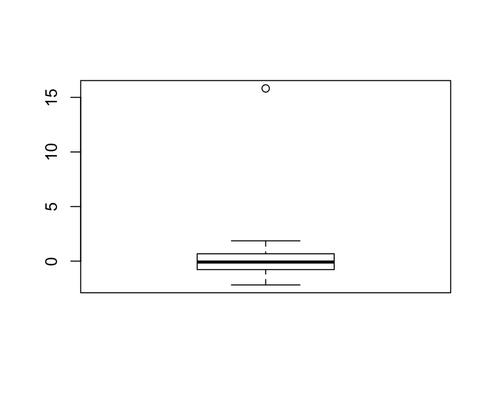
str(bxplt)## List of 6
## $ stats: num [1:5, 1] -2.1787 -0.773 -0.0829 0.6742 1.8609
## $ n : num 100
## $ conf : num [1:2, 1] -0.312 0.146
## $ out : num 15.8
## $ group: num 1
## $ names: chr "1"The str() function shows us the structure of the boxplot() output object. On inspection, you can see that the $out element of the list returned by the function includes the outlying values. The one we imputed manually (15.82) is there, which is a good sanity check. Let’s extract only these values:
outl <- boxplot(x, plot = F)$out # don't show plot
outl
## [1] 15.82Cool, all we need to do now is replace the values of x that are equal to these values with NAs:
x %in% outl## [1] FALSE FALSE FALSE FALSE FALSE FALSE FALSE FALSE FALSE FALSE FALSE
## [12] FALSE FALSE FALSE FALSE FALSE FALSE FALSE FALSE FALSE FALSE FALSE
## [23] FALSE FALSE FALSE FALSE FALSE FALSE FALSE FALSE FALSE FALSE FALSE
## [34] FALSE FALSE FALSE FALSE FALSE FALSE FALSE FALSE FALSE FALSE FALSE
## [45] FALSE FALSE FALSE FALSE FALSE FALSE FALSE FALSE FALSE FALSE FALSE
## [56] FALSE FALSE FALSE FALSE FALSE FALSE FALSE FALSE FALSE FALSE FALSE
## [67] FALSE FALSE FALSE FALSE FALSE FALSE FALSE FALSE FALSE FALSE FALSE
## [78] FALSE FALSE FALSE FALSE TRUE FALSE FALSE FALSE FALSE FALSE FALSE
## [89] FALSE FALSE FALSE FALSE FALSE FALSE FALSE FALSE FALSE FALSE FALSE
## [100] FALSEx[x %in% outl] <- NAWe can now look at x to see that the outlying values have been replaced with NAs:
x## [1] 0.55003837 -1.42600310 1.86086102 0.61658722 -0.01989037
## [6] -1.54940919 -0.09212116 -0.11995062 0.46371556 -0.21538979
## [11] 0.79616513 0.64245457 -1.53072648 0.07156453 -0.04578202
## [16] -1.97228003 -1.09441721 -1.13025339 0.58228972 0.82577526
## [21] 0.92187086 1.20341394 -0.52137727 -1.20640346 0.32866837
## [26] -1.29209019 -0.70846562 -1.37860020 1.30037578 0.56146544
## [31] -1.29017858 -0.24479689 -0.42077128 0.83924758 -0.83879491
## [36] -0.01883293 -0.43676928 0.25908625 0.79195701 0.84210433
## [41] -0.93341681 0.40779902 -1.99875332 -0.83749900 0.23358481
## [46] -0.23453260 1.19833978 -1.05011164 1.37827034 1.26252123
## [51] -1.67795023 0.70596056 -0.62086954 -0.21070733 -0.05602700
## [56] -0.11626018 -0.01266982 -0.58095453 1.21003452 -1.26289245
## [61] -1.43797434 -0.60246134 -0.68738194 -1.03864580 0.89307736
## [66] 0.15908639 -1.11950575 -0.36445912 -0.68091244 -0.38044496
## [71] 0.96545064 -0.18876035 0.83780059 0.09757592 -0.22836091
## [76] -2.17866447 1.16941126 0.43622198 -0.37805842 0.96286696
## [81] 1.49256410 NA -0.26050179 -1.07595095 -0.07363494
## [86] -0.52752823 0.15663362 -0.46795306 0.49035197 -1.07008923
## [91] 1.40284226 1.08135247 -0.40824955 -0.93838890 0.59133313
## [96] 0.91905183 1.51313338 0.07362568 -0.97509457 0.54023784Great! Now that we know our algorithm for removing outliers, we can write our function:
out.liar <- function(variable) { # arguments can be called whatever
  remove <- boxplot(variable, plot = F)$out
  variable[variable %in% remove] <- NA
  return(variable)
}
Let’s try it out!
x <- rnorm(20, 9, 2)
x[2] <- 1520
x
## [1] 8.390142 1520.000000 9.631565 14.557650 9.087212
## [6] 9.309832 10.237032 9.142086 7.549114 7.244644
## [11] 8.957332 7.890857 10.256586 10.429819 8.289764
## [16] 9.058645 12.604445 9.625969 8.693368 7.409008x <- out.liar(x)
x## [1] 8.390142 NA 9.631565 NA 9.087212 9.309832 10.237032
## [8] 9.142086 7.549114 7.244644 8.957332 7.890857 10.256586 10.429819
## [15] 8.289764 9.058645 12.604445 9.625969 8.693368 7.409008Pretty neat, huh?
The code inside of the function definition can be as simple or as complicated as you want it to be. However, it must run without errors and you need to think about various edge cases that might break the code or lead to unexpected behaviour. For instance, if we give out out.liar() function a character vector, it will throw an error because boxplot() can only cope with numeric vectors:
out.liar(letters)## Error in x[floor(d)] + x[ceiling(d)]: non-numeric argument to binary operatorThis error message is a little obscure but what happened is that out.liar() passed the vector of letters to boxplot() which, in turn, passed it to the + function. Since you cannot add letters, the function threw an error, thus breaking boxplot() and out.liar().
You might also wish to make the function able to identify outliers in a data frame. To do that you would have to make the function recognise which columns of the data frame provided are numeric and then run the code on each one of these columns. Finally the function should return the entire data frame with the non-numeric columns untouched and the numeric ones modified:
out.liar <- function(variable) { # arguments can be called whatever
  if (class(variable) == "data.frame") {
    # identify numeric variables by applying the is.numeric
    # function to each column of the data frame
    num_vars <- unlist(lapply(variable, is.numeric))
    # run the out.liar function on each numeric column
    # this kind of recurrence where you run a function inside of itself
    # is allowed and often used!
    variable[num_vars] <- lapply(variable[num_vars], out.liar)
  } else {
    remove <- boxplot(variable, plot = F)$out
    variable[variable %in% remove] <- NA
  }
  return(variable)
}
Let’s see if it works. First, create some data frame with a couple of outlying values:
df <- data.frame(id = factor(1:10), var1 = c(100, rnorm(9)),
                 var2 = c(rchisq(9, 4), 100), var3 = LETTERS[1:10])
df
## id var1 var2 var3
## 1 1 100.00000000 3.9174945 A
## 2 2 0.47461824 2.5883314 B
## 3 3 -1.76634605 1.6285662 C
## 4 4 -0.04140268 3.5953417 D
## 5 5 -0.74529598 8.3492440 E
## 6 6 0.55631124 0.2957526 F
## 7 7 0.57117284 2.8894209 G
## 8 8 2.92466663 12.4805552 H
## 9 9 0.45180224 2.5062931 I
## 10 10 -1.31348905 100.0000000 JNext, feed df to out.liar():
out.liar(df)## id var1 var2 var3
## 1 1 NA 3.9174945 A
## 2 2 0.47461824 2.5883314 B
## 3 3 -1.76634605 1.6285662 C
## 4 4 -0.04140268 3.5953417 D
## 5 5 -0.74529598 8.3492440 E
## 6 6 0.55631124 0.2957526 F
## 7 7 0.57117284 2.8894209 G
## 8 8 NA 12.4805552 H
## 9 9 0.45180224 2.5062931 I
## 10 10 -1.31348905 NA JFinally, check if the function still works on single columns even after our modification:
x <- rnorm(20, 9, 2)
x[2] <- 1520
out.liar(x)
## [1] 11.227530 NA 11.122428 9.046352 9.047519 9.011521 5.715875
## [8] 7.355825 8.852045 10.386154 7.597622 8.540947 6.287205 8.310314
## [15] 7.004540 11.916455 11.264865 10.769398 5.298348 7.785135Everything looking good!
So this is how you write functions. The principle is simple but actually creating good and safe functions requires a lot of thinking and attention to detail.
6.4.3.1 Hacking
Finally, if you’re really into the nitty-gritty of R, a great way of learning how to write functions is to look at ones you use and try to pick them apart, break them, fix them, and put them back together.
Since – sing along – everything in R is an object, you can assign the code inside of an already existing function to some other object. For instance, the boxplot() function calls a different “method” based on what input you give it (this is rather advanced programming so don’t worry too much about it!). The one we used is called botplot.default() and it hides deep inside package "graphics". To get it out, we need to tell R to get it from there using the package:::function syntax:
box2 <- graphics:::boxplot.default
box2
## function (x, ..., range = 1.5, width = NULL, varwidth = FALSE,
## notch = FALSE, outline = TRUE, names, plot = TRUE, border = par("fg"),
## col = NULL, log = "", pars = list(boxwex = 0.8, staplewex = 0.5,
## outwex = 0.5), horizontal = FALSE, add = FALSE, at = NULL)
## {
## args <- list(x, ...)
## namedargs <- if (!is.null(attributes(args)$names))
## attributes(args)$names != ""
## else rep_len(FALSE, length(args))
## groups <- if (is.list(x))
## x
## else args[!namedargs]
## if (0L == (n <- length(groups)))
## stop("invalid first argument")
## if (length(class(groups)))
## groups <- unclass(groups)
## if (!missing(names))
## attr(groups, "names") <- names
## else {
## if (is.null(attr(groups, "names")))
## attr(groups, "names") <- 1L:n
## names <- attr(groups, "names")
## }
## cls <- vapply(groups, function(x) class(x)[1L], "")
## cl <- if (all(cls == cls[1L]))
## cls[1L]
## for (i in 1L:n) groups[i] <- list(boxplot.stats(unclass(groups[[i]]),
## range))
## stats <- matrix(0, nrow = 5L, ncol = n)
## conf <- matrix(0, nrow = 2L, ncol = n)
## ng <- out <- group <- numeric(0L)
## ct <- 1
## for (i in groups) {
## stats[, ct] <- i$stats
## conf[, ct] <- i$conf
## ng <- c(ng, i$n)
## if ((lo <- length(i$out))) {
## out <- c(out, i$out)
## group <- c(group, rep.int(ct, lo))
## }
## ct <- ct + 1
## }
## if (length(cl) && cl != "numeric")
## oldClass(stats) <- cl
## z <- list(stats = stats, n = ng, conf = conf, out = out,
## group = group, names = names)
## if (plot) {
## if (is.null(pars$boxfill) && is.null(args$boxfill))
## pars$boxfill <- col
## do.call("bxp", c(list(z, notch = notch, width = width,
## varwidth = varwidth, log = log, border = border,
## pars = pars, outline = outline, horizontal = horizontal,
## add = add, at = at), args[namedargs]))
## invisible(z)
## }
## else z
## }
## <bytecode: 0x7f9087125f60>
## <environment: namespace:graphics>This is the code that creates the boxplot and, if you wish, you can try to look into it and find how the function identifies outliers. You can even change the function by typing edit(box2).
Being able to peer under the hood of readymade functions opens up an infinite playground for you so enjoy yourself!