Chapter 15 Linear Model and Mixed Methods
Note: this section is partically adapted from Fox (2002), Linear Mixed Models and Bates et al (2015) . We will frist focus on simple linear model, we extend it to fixed effect model, finally we discuss random effects modelling. We will alose use the data from study of Belenky et al (2003). This is pretty famous dataset that is easy to find online and you may find some help on it easily as many people are using it either to teach or to learn about random effects.
15.1 Longitudinal Data
We have seen quite a few examples of linear models earlier this week, let us now finally get to the ones you probably came here to learn more about. The world can be slighlty more complex of course than traditional set up of linear models. Things change in time and they change differently for differnt units of analysis. We want to control for the variation in this change when making claims about casual relationship we find using data. In psychological research, especially, you often find that you will have some repeated measures of your variable of interest for participants (i.e. memory after perfoming certain tests, reaction scores, attitudes, etc). These are realted either to multiple treatments given to participatns of measuring the same relationships at different time points.
Remember old model set up: \[\begin{equation} Y_[i] = \beta_0 + \beta_1 * X_i + \epsilon_i \end{equation}\]
And remember the assumptions that are required for the linear model Once in repeated measures setting you will see that most of these will remain. As in the simple linear model,we do care most about our residual term. We want it to be random and normally distributed with zero mean. The main reason for that of course is the fact that we want our model to explain all the meaningful variations without leaving anything in the residual term.
The only difference we have now is the we want to control for each individual unobserved characteristics so we introduce extra parameter which will account for those.
\[\begin{equation} Y_[i] = \beta_0 + \beta_1 * X_i + \alpha + \epsilon_i \end{equation}\]
This is the fixed effect model.
We can also introduce further parameters that will allows us to include effects at individual levels (i.e. pupils) and at the entity levels (i.e.schools)
\[\begin{equation} Y_[i] = \beta_0 + \beta_1 * X_i + \theta_i + \gamma_ij + \epsilon_i \end{equation}\]
15.2 Why do we do this?
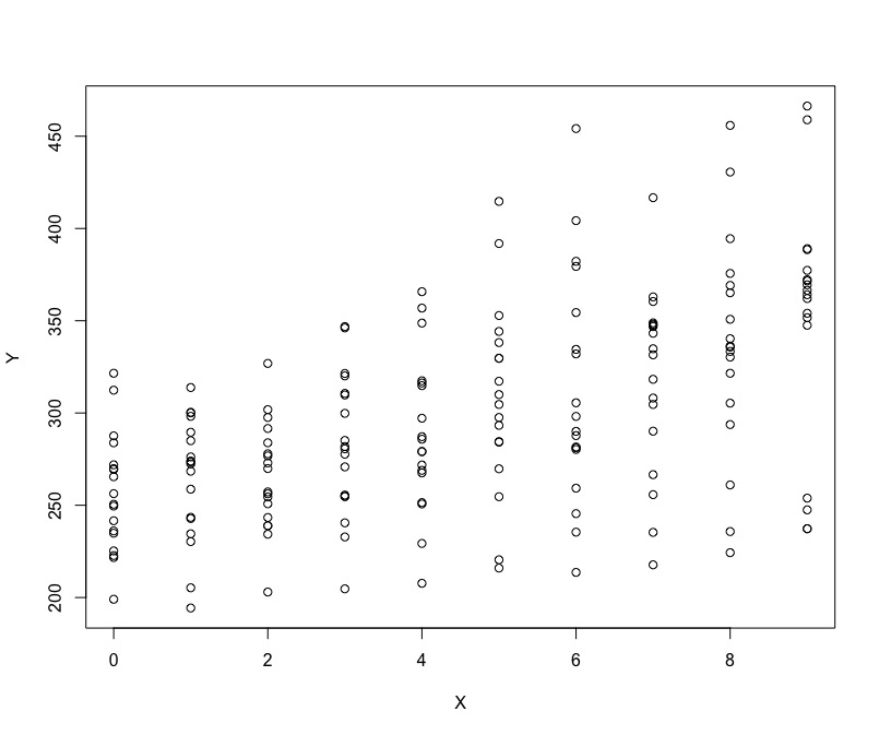
The reason why we are introducing a new model for repeated measures data or data that has few levels is the consideration of Ecological fallacy. What do we mean by that is that there may be differences across the effects on the levels of units compared to that on individual levels. Lets look at the example of the data:
Do you think we have positive relationship or negative? is it easy to tell what is happening?
15.3 Ecological Fallacy (quick illustration)
Lets get some data in and load lmer package:
library(lme4)
disease<-read.csv('disease.csv')
We will run three models:
#Not controlling for city
model_0 <- lm(HDisease~Income, data = disease)
#Controlling for city effects
model_1 <- lm(HDisease~Income+factor(City), data = disease)
#Controlling for city and across cities effects
model_2 <- lmer(HDisease~Income + (1 | City), data = disease)
Lets compare the outputs:
library(texreg)
screenreg(list(model_0, model_1, model_2))
##
## =========================================================
## Model 1 Model 2 Model 3
## ---------------------------------------------------------
## (Intercept) 1.65 *** 3.07 *** 16.41 ***
## (0.27) (0.11) (2.87)
## Income 1.95 *** -0.99 *** -0.98 ***
## (0.05) (0.07) (0.07)
## factor(City)2 2.88 ***
## (0.16)
## factor(City)3 5.96 ***
## (0.21)
## factor(City)4 8.91 ***
## (0.26)
## factor(City)5 12.06 ***
## (0.33)
## factor(City)6 14.89 ***
## (0.40)
## factor(City)7 17.78 ***
## (0.47)
## factor(City)8 20.90 ***
## (0.54)
## factor(City)9 23.86 ***
## (0.59)
## factor(City)10 26.93 ***
## (0.68)
## ---------------------------------------------------------
## R^2 0.95 1.00
## Adj. R^2 0.95 1.00
## Num. obs. 100 100 100
## RMSE 1.34 0.32
## AIC 148.61
## BIC 159.03
## Log Likelihood -70.31
## Num. groups: City 10
## Var: City (Intercept) 81.14
## Var: Residual 0.10
## =========================================================
## *** p < 0.001, ** p < 0.01, * p < 0.0515.4 Simple model
Lets load all the packages we will need:
library(lattice)
library(arm)
We will use the data on sleep deprivation. The example is based on Belenky et al (2003) study that looks at patterns of sleeping across individuals that are doing through the stages of sleep deprivation. On day 0 the subjects had their normal amount of sleep. Starting that night they were restricted to 3 hours of sleep per night. The observations represent the average reaction time on a series of tests given each day to each subject.
sleep<-read.csv('sleep.csv')Lets just plot the data as it is. We will use Days as our X, and reaction as our Y. You will recognize something we just have seen.
qplot(sleep$Days, sleep$Reaction, xlab='Days', ylab='Reaction')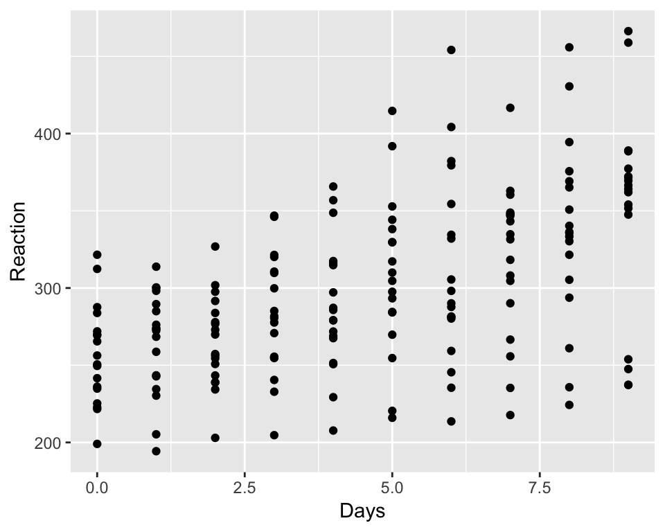
It is a hard to tell whether there is a positive effect or whether there may be different levels of effect, it is clearly that there is some tendency for increasing reaction as time passes but we have various individuals we may find that on individual levels we may observe a more detailed picture.
We can use xy plot to plot the variation of reaction time for the test which were given to participants across ten days of the recovery.
xyplot(Reaction ~ Days|Subject, sleep, type = c("g","p","r"),
       index = function(x,y) coef(lm(y ~ x))[1],
       xlab = "Days of sleep deprivation",
       ylab = "Average reaction time (ms)", aspect = "xy")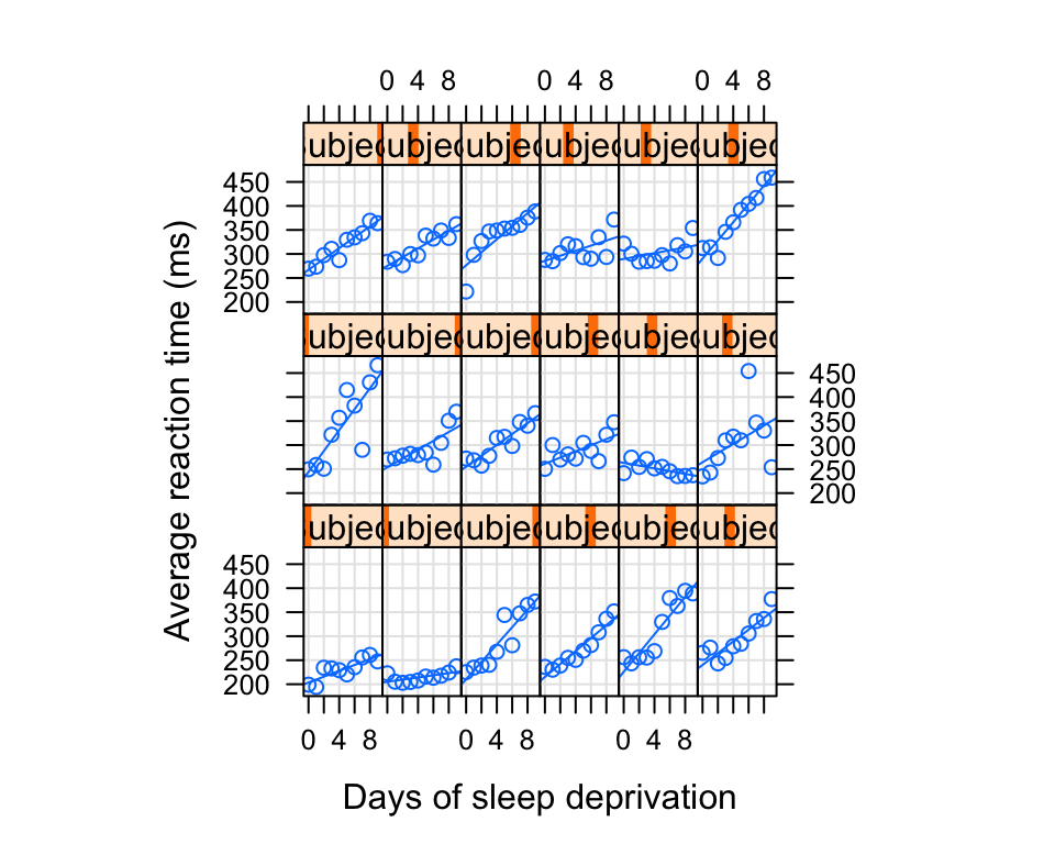
What do you see? It looks like for some individuals there were pretty fast changes in the reactions times across periods with some having steady growth in reaction level.
Note how in the plots I included the variables Days|Subject, sleep. This helps to identify that we are looking at the effect of time for each subject’s sleep variable.
Let us now see if we were to run a model to fit this data.
15.4.1 Pooling
We can start with simple model, this is also know as complete polling, we assume that effects of variable Day were the same for everyone.
model_simple<-lm(Reaction~Days, sleep)

summary(model_simple)
##
## Call:
## lm(formula = Reaction ~ Days, data = sleep)
##
## Residuals:
## Min 1Q Median 3Q Max
## -110.848 -27.483 1.546 26.142 139.953
##
## Coefficients:
## Estimate Std. Error t value Pr(>|t|)
## (Intercept) 251.405 6.610 38.033 < 2e-16 ***
## Days 10.467 1.238 8.454 9.89e-15 ***
## ---
## Signif. codes: 0 '***' 0.001 '**' 0.01 '*' 0.05 '.' 0.1 ' ' 1
##
## Residual standard error: 47.71 on 178 degrees of freedom
## Multiple R-squared: 0.2865, Adjusted R-squared: 0.2825
## F-statistic: 71.46 on 1 and 178 DF, p-value: 9.894e-1515.4.2 No pooling
We can also control for each subject, this is known as fixed effect and is equivalent to having a dummy variable for each of the individuals:
model_subject<-lm(Reaction~Days+as.factor(Subject), sleep)

summary(model_subject)
##
## Call:
## lm(formula = Reaction ~ Days + as.factor(Subject), data = sleep)
##
## Residuals:
## Min 1Q Median 3Q Max
## -100.540 -16.389 -0.341 15.215 131.159
##
## Coefficients:
## Estimate Std. Error t value Pr(>|t|)
## (Intercept) 295.0310 10.4471 28.240 < 2e-16 ***
## Days 10.4673 0.8042 13.015 < 2e-16 ***
## as.factor(Subject)309 -126.9008 13.8597 -9.156 2.35e-16 ***
## as.factor(Subject)310 -111.1326 13.8597 -8.018 2.07e-13 ***
## as.factor(Subject)330 -38.9124 13.8597 -2.808 0.005609 **
## as.factor(Subject)331 -32.6978 13.8597 -2.359 0.019514 *
## as.factor(Subject)332 -34.8318 13.8597 -2.513 0.012949 *
## as.factor(Subject)333 -25.9755 13.8597 -1.874 0.062718 .
## as.factor(Subject)334 -46.8318 13.8597 -3.379 0.000913 ***
## as.factor(Subject)335 -92.0638 13.8597 -6.643 4.51e-10 ***
## as.factor(Subject)337 33.5872 13.8597 2.423 0.016486 *
## as.factor(Subject)349 -66.2994 13.8597 -4.784 3.87e-06 ***
## as.factor(Subject)350 -28.5311 13.8597 -2.059 0.041147 *
## as.factor(Subject)351 -52.0361 13.8597 -3.754 0.000242 ***
## as.factor(Subject)352 -4.7123 13.8597 -0.340 0.734300
## as.factor(Subject)369 -36.0992 13.8597 -2.605 0.010059 *
## as.factor(Subject)370 -50.4321 13.8597 -3.639 0.000369 ***
## as.factor(Subject)371 -47.1498 13.8597 -3.402 0.000844 ***
## as.factor(Subject)372 -24.2477 13.8597 -1.750 0.082108 .
## ---
## Signif. codes: 0 '***' 0.001 '**' 0.01 '*' 0.05 '.' 0.1 ' ' 1
##
## Residual standard error: 30.99 on 161 degrees of freedom
## Multiple R-squared: 0.7277, Adjusted R-squared: 0.6973
## F-statistic: 23.91 on 18 and 161 DF, p-value: < 2.2e-16We can test whether controlling for each individual variation improves on a simple model:
anova(model_simple, model_subject)## Analysis of Variance Table
##
## Model 1: Reaction ~ Days
## Model 2: Reaction ~ Days + as.factor(Subject)
## Res.Df RSS Df Sum of Sq F Pr(>F)
## 1 178 405252
## 2 161 154634 17 250618 15.349 < 2.2e-16 ***
## ---
## Signif. codes: 0 '***' 0.001 '**' 0.01 '*' 0.05 '.' 0.1 ' ' 1However you should note that in this structure we do not consider anything with regards to between units variation, we are looking at what happening within individuals reaction but do not compare them
15.4.3 Partial Pooling (varying intercepts)
An attempt do so can be using random effect modelling structure. This will first look at the variation between individuals and then measure their distance from average individual effect, so we are partially pooling everyone together. Please note that we are assuming the slopes are the same, it is the intercepts that will vary for each person.
#Run baseline model (will use it later for comparison, we have  no controls)
model_null <- lmer(Reaction ~  (1|Subject) , sleep)


#Run the model (note thay we also control for the effect of time by subject)
model_mix <- lmer(Reaction ~ Days + (1|Subject) , sleep)
#Summarise
summary(model_mix)
## Linear mixed model fit by REML ['lmerMod']
## Formula: Reaction ~ Days + (1 | Subject)
## Data: sleep
##
## REML criterion at convergence: 1786.5
##
## Scaled residuals:
## Min 1Q Median 3Q Max
## -3.2257 -0.5529 0.0109 0.5188 4.2506
##
## Random effects:
## Groups Name Variance Std.Dev.
## Subject (Intercept) 1378.2 37.12
## Residual 960.5 30.99
## Number of obs: 180, groups: Subject, 18
##
## Fixed effects:
## Estimate Std. Error t value
## (Intercept) 251.4051 9.7467 25.79
## Days 10.4673 0.8042 13.02
##
## Correlation of Fixed Effects:
## (Intr)
## Days -0.371Double check that the intercept for fixed effect is identical to the one we found earlier when we controlled for the subject. The coefficient for ‘Days’ reports the average effect of an extra day of sleep deprivation on reaction score.
Lets get to a bit more detailed output:
display(model_mix)## lmer(formula = Reaction ~ Days + (1 | Subject), data = sleep)
## coef.est coef.se
## (Intercept) 251.41 9.75
## Days 10.47 0.80
##
## Error terms:
## Groups Name Std.Dev.
## Subject (Intercept) 37.12
## Residual 30.99
## ---
## number of obs: 180, groups: Subject, 18
## AIC = 1794.5, DIC = 1801.7
## deviance = 1794.1We can extract fixed effect estimation:
fixef(model_mix) ## (Intercept) Days
## 251.40510 10.46729se.fixef(model_mix)## (Intercept) Days
## 9.7467163 0.8042214Or random effect:
ranef(model_mix)## $Subject
## (Intercept)
## 308 40.783710
## 309 -77.849554
## 310 -63.108567
## 330 4.406442
## 331 10.216189
## 332 8.221238
## 333 16.500494
## 334 -2.996981
## 335 -45.282127
## 337 72.182686
## 349 -21.196249
## 350 14.111363
## 351 -7.862221
## 352 36.378425
## 369 7.036381
## 370 -6.362703
## 371 -3.294273
## 372 18.115747
##
## with conditional variances for "Subject"se.ranef(model_mix)## $Subject
## (Intercept)
## 308 9.475668
## 309 9.475668
## 310 9.475668
## 330 9.475668
## 331 9.475668
## 332 9.475668
## 333 9.475668
## 334 9.475668
## 335 9.475668
## 337 9.475668
## 349 9.475668
## 350 9.475668
## 351 9.475668
## 352 9.475668
## 369 9.475668
## 370 9.475668
## 371 9.475668
## 372 9.47566815.4.4 Partial Pooling (varying intercepts and/or slopes)
We can also vary slopes if we wanted to, we saw earlier that we may have very different line fit for reaction time for different individuals.
#Run the model (note thay we also control for the effect of time by subject)
model_mix_slope <- lmer(Reaction ~ Days + (Days|Subject) , sleep)
#Summarise
summary(model_mix_slope)
## Linear mixed model fit by REML ['lmerMod']
## Formula: Reaction ~ Days + (Days | Subject)
## Data: sleep
##
## REML criterion at convergence: 1743.6
##
## Scaled residuals:
## Min 1Q Median 3Q Max
## -3.9536 -0.4634 0.0231 0.4633 5.1793
##
## Random effects:
## Groups Name Variance Std.Dev. Corr
## Subject (Intercept) 611.90 24.737
## Days 35.08 5.923 0.07
## Residual 654.94 25.592
## Number of obs: 180, groups: Subject, 18
##
## Fixed effects:
## Estimate Std. Error t value
## (Intercept) 251.405 6.824 36.843
## Days 10.467 1.546 6.771
##
## Correlation of Fixed Effects:
## (Intr)
## Days -0.138Each subject now will have their own slope estimation, which is as intercept is partially pooled towards the center of days effects distribution. Note the results for days coefficients in the main output.
Whatever decision you make, it will always be driven by your data. You may want to do model comparison and analysis the residuals in model output to see how much varying intercepts/slopes improved your understanding of underlying relationships in your data.
We can use log likelihood ratio test to compare the models we just built:
#Make sure lmtest is loaded
library(lmtest)
#Compare the null model with random intercept model
lrtest(model_null,model_mix)## Likelihood ratio test
##
## Model 1: Reaction ~ (1 | Subject)
## Model 2: Reaction ~ Days + (1 | Subject)
## #Df LogLik Df Chisq Pr(>Chisq)
## 1 3 -952.16
## 2 4 -893.23 1 117.86 < 2.2e-16 ***
## ---
## Signif. codes: 0 '***' 0.001 '**' 0.01 '*' 0.05 '.' 0.1 ' ' 1#Now varying intercept with both varying interecept + slopes
lrtest(model_mix, model_mix_slope)## Likelihood ratio test
##
## Model 1: Reaction ~ Days + (1 | Subject)
## Model 2: Reaction ~ Days + (Days | Subject)
## #Df LogLik Df Chisq Pr(>Chisq)
## 1 4 -893.23
## 2 6 -871.81 2 42.837 4.99e-10 ***
## ---
## Signif. codes: 0 '***' 0.001 '**' 0.01 '*' 0.05 '.' 0.1 ' ' 1The model with random intercept improves on null model. Having a random slope and intercept improved the model even more.
We can also use something which is known pseudo R squared to see how much variance was explained due to our explanatory factor. We will need to calculate it by hand. We will use our model without controls where were have random intercepts and we will add days to compare the explained variation that is due to addition of explanatory factors. Just a reminder of the models we need:
model_null <- lmer(Reaction ~  (1|Subject) , sleep)
model_mix <- lmer(Reaction ~ Days + (1|Subject) , sleep)
## We can try to extract the partial variance that was explained by Days for mixed model
totvar_model_null <- (summary(model_null)$sigma)^2 + as.numeric(summary(model_null)$varcor)
totvar_model_mix <- (summary(model_mix)$sigma)^2 + as.numeric(summary(model_mix)$varcor)
Var_expl <-(totvar_model_null-totvar_model_mix)/totvar_model_null
Var_expl## [1] 0.2775756We find that about 28% of variation in reaction can be explained by time, when controlling for subjects.
Lets finally put all these models side by side:
#Make sure to have textreg loaded
library(texreg)screenreg(list(model_null, model_mix))##
## ==================================================
## Model 1 Model 2
## --------------------------------------------------
## (Intercept) 298.51 *** 251.41 ***
## (9.05) (9.75)
## Days 10.47 ***
## (0.80)
## --------------------------------------------------
## AIC 1910.33 1794.47
## BIC 1919.91 1807.24
## Log Likelihood -952.16 -893.23
## Num. obs. 180 180
## Num. groups: Subject 18 18
## Var: Subject (Intercept) 1278.34 1378.18
## Var: Residual 1958.87 960.46
## ==================================================
## *** p < 0.001, ** p < 0.01, * p < 0.0515.5 Multilevel modelling with random intercepts and slopes
Multilevel models are used for cases where there are few levels to the measurement. A very common way to illustrate this is using students grades across schools that vary within the pupils at the school but also vary across schools. This is relevant in cases where grades were measure in different times as well.
For studies that look at this closely have a look at this review paper. The data set that we will work with has information on IQ scores for school students and is taken from Snijders and Bosker (2012) textbook. We will have different levels here, variability of grades within the schools and across the schools. What we want to understand is whether average score on languge test has anything to do with scores that student get in their SES and IQ and the scores at the average school level.
school: School id pupil: Student id lang_score: language score ses:Socioeconomic status of the student (mean centered) IQ_verb: Verbal IQ of the student (mean centered) sex: Gender of the student Minority: Dummy indicator of whether student is of minority background sch_ses: Average SES in a school (mean centered) sch_iqv: Average verbal IQ in a school (mean centered) sch_min: Proportion of minority students in a school
15.5.1 Prepare
Before we start let us load all the packages we will need later.
library(nlme)
library(lattice)schools<-read.csv('schools.csv')
head(schools)## school pupil lang_score ses IQ_verb sex Minority sch_ses sch_iqv
## 1 1 3 46 -4.73 3.13 0 0 -14.035 -1.4039
## 2 1 4 45 -17.73 2.63 0 1 -14.035 -1.4039
## 3 1 5 33 -12.73 -2.37 0 0 -14.035 -1.4039
## 4 1 6 46 -4.73 -0.87 0 0 -14.035 -1.4039
## 5 1 7 20 -17.73 -3.87 0 0 -14.035 -1.4039
## 6 1 8 30 -17.73 -2.37 0 1 -14.035 -1.4039
## sch_min
## 1 0.63
## 2 0.63
## 3 0.63
## 4 0.63
## 5 0.63
## 6 0.63Let us first build a simple mixed effect model, we will try to predict language scores and will control for the school only:
model_schools_0 <- lmer(lang_score ~  (1|school), data = schools)
summary(model_schools_0)
## Linear mixed model fit by REML ['lmerMod']
## Formula: lang_score ~ (1 | school)
## Data: schools
##
## REML criterion at convergence: 26595.7
##
## Scaled residuals:
## Min 1Q Median 3Q Max
## -4.1850 -0.6417 0.0905 0.7226 2.5281
##
## Random effects:
## Groups Name Variance Std.Dev.
## school (Intercept) 18.24 4.271
## Residual 62.85 7.928
## Number of obs: 3758, groups: school, 211
##
## Fixed effects:
## Estimate Std. Error t value
## (Intercept) 41.0038 0.3257 125.9We can also set up a NULL model, explained variance of which we will use to calculate pseudo R squared:
model_schools_null<- lm(lang_score ~1, data = schools)
summary(model_schools_null)
##
## Call:
## lm(formula = lang_score ~ 1, data = schools)
##
## Residuals:
## Min 1Q Median 3Q Max
## -33.413 -5.413 0.587 6.587 16.587
##
## Coefficients:
## Estimate Std. Error t value Pr(>|t|)
## (Intercept) 41.4130 0.1451 285.5 <2e-16 ***
## ---
## Signif. codes: 0 '***' 0.001 '**' 0.01 '*' 0.05 '.' 0.1 ' ' 1
##
## Residual standard error: 8.893 on 3757 degrees of freedomWe can quickly check whether having varying intercepts improves over having a single one for everyone:
lrtest(model_schools_null,model_schools_0)## Likelihood ratio test
##
## Model 1: lang_score ~ 1
## Model 2: lang_score ~ (1 | school)
## #Df LogLik Df Chisq Pr(>Chisq)
## 1 2 -13544
## 2 3 -13298 1 492.54 < 2.2e-16 ***
## ---
## Signif. codes: 0 '***' 0.001 '**' 0.01 '*' 0.05 '.' 0.1 ' ' 1Lets start adding some covariates, we can start with IQ and then see how much additional variance can be explained by the variable:
model_schools_IQ <- lmer(lang_score ~ IQ_verb + (1|school), data = schools, REML =FALSE)
summary(model_schools_IQ)
## Linear mixed model fit by maximum likelihood ['lmerMod']
## Formula: lang_score ~ IQ_verb + (1 | school)
## Data: schools
##
## AIC BIC logLik deviance df.resid
## 24920.2 24945.1 -12456.1 24912.2 3754
##
## Scaled residuals:
## Min 1Q Median 3Q Max
## -4.1963 -0.6385 0.0659 0.7098 3.2143
##
## Random effects:
## Groups Name Variance Std.Dev.
## school (Intercept) 9.845 3.138
## Residual 40.469 6.362
## Number of obs: 3758, groups: school, 211
##
## Fixed effects:
## Estimate Std. Error t value
## (Intercept) 41.05488 0.24339 168.68
## IQ_verb 2.50744 0.05438 46.11
##
## Correlation of Fixed Effects:
## (Intr)
## IQ_verb 0.003Lets calculate variance of empty model, then with IQ:
totvar_model_0 <- (summary(model_schools_0)$sigma)^2 + as.numeric(summary(model_schools_0)$varcor)

totvar_model_IQ <- (summary(model_schools_IQ)$sigma)^2 + as.numeric(summary(model_schools_IQ)$varcor)

# Proportion of variance explained by IQ:

Rsq_IQ <- (totvar_model_0 - totvar_model_IQ)/totvar_model_0

Rsq_IQ
## [1] 0.3795199On top of that, we can also make assessment of intraclass correlation (ICC), this will allow us to investigate whether there are systematic similarities in grades within the schools.
Lets get one for our first model:
ICC_0 <- as.numeric(summary(model_schools_0)$varcor)/((summary(model_schools_0)$sigma)^2 + as.numeric(summary(model_schools_0)$varcor))
ICC_0
## [1] 0.2249341This tell us that about 22 percent of variation in language scores is at the school level. This can also be stated as the following: if we picked randomly two students that belong to the same school, we would expect about 0.22 correlation in their language scores.
ICC_IQ<-as.numeric(summary(model_schools_IQ)$varcor)/((summary(model_schools_IQ)$sigma)^2 + as.numeric(summary(model_schools_IQ)$varcor))
ICC_IQ
## [1] 0.1956726We dropped to to 0.2 now, this tell us that once we look at the similarity of IQ scores at the school level, the correlation between the scores obtained on lang score can be explained by similarities in IQ scores within the school.
Finally, lets now add the schools average scores dynamic to our model:
model_schools_IQ_sc <- lmer(lang_score ~ IQ_verb + sch_iqv + (1|school), data = schools, REML =FALSE)
summary(model_schools_IQ_sc)
## Linear mixed model fit by maximum likelihood ['lmerMod']
## Formula: lang_score ~ IQ_verb + sch_iqv + (1 | school)
## Data: schools
##
## AIC BIC logLik deviance df.resid
## 24898.0 24929.2 -12444.0 24888.0 3753
##
## Scaled residuals:
## Min 1Q Median 3Q Max
## -4.2220 -0.6411 0.0634 0.7059 3.2190
##
## Random effects:
## Groups Name Variance Std.Dev.
## school (Intercept) 8.68 2.946
## Residual 40.43 6.358
## Number of obs: 3758, groups: school, 211
##
## Fixed effects:
## Estimate Std. Error t value
## (Intercept) 41.11378 0.23181 177.362
## IQ_verb 2.45361 0.05549 44.218
## sch_iqv 1.31242 0.26160 5.017
##
## Correlation of Fixed Effects:
## (Intr) IQ_vrb
## IQ_verb -0.007
## sch_iqv 0.043 -0.210Try to get ICC and R squared by yourself here. You will find that controlling for average IQ in the school will improve model as well. We can thus incorporate the school levels on top of individual level of the final model and perform a likelihood ratio test.
model_school_final <- lmer(lang_score ~ IQ_verb + sch_iqv + (1+IQ_verb|school),
           data = schools, REML =FALSE)
summary(model_school_final)
## Linear mixed model fit by maximum likelihood ['lmerMod']
## Formula: lang_score ~ IQ_verb + sch_iqv + (1 + IQ_verb | school)
## Data: schools
##
## AIC BIC logLik deviance df.resid
## 24878.9 24922.5 -12432.4 24864.9 3751
##
## Scaled residuals:
## Min 1Q Median 3Q Max
## -4.2615 -0.6335 0.0677 0.7033 2.7619
##
## Random effects:
## Groups Name Variance Std.Dev. Corr
## school (Intercept) 8.8783 2.9796
## IQ_verb 0.1949 0.4415 -0.63
## Residual 39.6855 6.2996
## Number of obs: 3758, groups: school, 211
##
## Fixed effects:
## Estimate Std. Error t value
## (Intercept) 41.12747 0.23363 176.036
## IQ_verb 2.47973 0.06429 38.569
## sch_iqv 1.02851 0.26221 3.923
##
## Correlation of Fixed Effects:
## (Intr) IQ_vrb
## IQ_verb -0.279
## sch_iqv -0.003 -0.188lrtest(model_schools_IQ_sc, model_school_final)## Likelihood ratio test
##
## Model 1: lang_score ~ IQ_verb + sch_iqv + (1 | school)
## Model 2: lang_score ~ IQ_verb + sch_iqv + (1 + IQ_verb | school)
## #Df LogLik Df Chisq Pr(>Chisq)
## 1 5 -12444
## 2 7 -12432 2 23.149 9.404e-06 ***
## ---
## Signif. codes: 0 '***' 0.001 '**' 0.01 '*' 0.05 '.' 0.1 ' ' 1Finally, as usual by now, lets put everything side by side:
screenreg(list(model_schools_0, model_schools_IQ, model_schools_IQ_sc, model_school_final))##
## ===========================================================================================
## Model 1 Model 2 Model 3 Model 4
## -------------------------------------------------------------------------------------------
## (Intercept) 41.00 *** 41.05 *** 41.11 *** 41.13 ***
## (0.33) (0.24) (0.23) (0.23)
## IQ_verb 2.51 *** 2.45 *** 2.48 ***
## (0.05) (0.06) (0.06)
## sch_iqv 1.31 *** 1.03 ***
## (0.26) (0.26)
## -------------------------------------------------------------------------------------------
## AIC 26601.69 24920.17 24898.02 24878.87
## BIC 26620.38 24945.09 24929.18 24922.49
## Log Likelihood -13297.84 -12456.08 -12444.01 -12432.44
## Num. obs. 3758 3758 3758 3758
## Num. groups: school 211 211 211 211
## Var: school (Intercept) 18.24 9.85 8.68 8.88
## Var: Residual 62.85 40.47 40.43 39.69
## Var: school IQ_verb 0.19
## Cov: school (Intercept) IQ_verb -0.83
## ===========================================================================================
## *** p < 0.001, ** p < 0.01, * p < 0.0515.6 Random slopes, intercepts and cross level interactions (optional)
For this part we will use the dataset taken from Hox’s (2010) textbook on multilevel modelling. The dataset includes the following variables:
PUPIL : pupil id within class CLASS : class id (1,…,100) POPULAR : popularity score of the student SEX : sex of the student (0=male, 1=female) T.EXP : years of experience of the theacher
popularity<-read.csv('Popularity.csv')We will go on straight to building our models, starting with null once again for later comparison.
model_null <- lm(POPULAR ~ 1, data = popularity)
model_pop_0 <- lmer(POPULAR ~ (1|CLASS), data = popularity)
summary(model_pop_0)
## Linear mixed model fit by REML ['lmerMod']
## Formula: POPULAR ~ (1 | CLASS)
## Data: popularity
##
## REML criterion at convergence: 5115.6
##
## Scaled residuals:
## Min 1Q Median 3Q Max
## -2.88825 -0.63376 -0.05155 0.71091 3.00393
##
## Random effects:
## Groups Name Variance Std.Dev.
## CLASS (Intercept) 0.8798 0.9380
## Residual 0.6387 0.7992
## Number of obs: 2000, groups: CLASS, 100
##
## Fixed effects:
## Estimate Std. Error t value
## (Intercept) 5.3076 0.0955 55.58Tst whether random intercepts is an improvement:
lrtest(model_pop_0,model_null)## Likelihood ratio test
##
## Model 1: POPULAR ~ (1 | CLASS)
## Model 2: POPULAR ~ 1
## #Df LogLik Df Chisq Pr(>Chisq)
## 1 3 -2557.8
## 2 2 -3244.8 -1 1373.9 < 2.2e-16 ***
## ---
## Signif. codes: 0 '***' 0.001 '**' 0.01 '*' 0.05 '.' 0.1 ' ' 1Lets see whether gender has anything to do with popularity:
model_pop_sex <- lmer(POPULAR ~ FEMALE+(1|CLASS), data = popularity)
summary(model_pop_sex)
## Linear mixed model fit by REML ['lmerMod']
## Formula: POPULAR ~ FEMALE + (1 | CLASS)
## Data: popularity
##
## REML criterion at convergence: 4492.9
##
## Scaled residuals:
## Min 1Q Median 3Q Max
## -3.3184 -0.6892 0.0018 0.5961 3.8239
##
## Random effects:
## Groups Name Variance Std.Dev.
## CLASS (Intercept) 0.8622 0.9286
## Residual 0.4599 0.6782
## Number of obs: 2000, groups: CLASS, 100
##
## Fixed effects:
## Estimate Std. Error t value
## (Intercept) 4.89722 0.09530 51.39
## FEMALETRUE 0.84370 0.03096 27.25
##
## Correlation of Fixed Effects:
## (Intr)
## FEMALETRUE -0.158## Pseudo R squared:
totvar_mod_pop_0 <- (summary(model_pop_0)$sigma)^2 + as.numeric(summary(model_pop_0)$varcor)
totvar_mod_pop_sex <- (summary(model_pop_sex)$sigma)^2 + as.numeric(summary(model_pop_sex)$varcor)
R_sq_pop <- (totvar_mod_pop_0 - totvar_mod_pop_sex)/totvar_mod_pop_0
R_sq_pop## [1] 0.1293066What about ICC?
as.numeric(summary(model_pop_sex)$varcor)/((summary(model_pop_sex)$sigma)^2 + as.numeric(summary(model_pop_sex)$varcor))## [1] 0.652142Lets add teching experience:
model_pop_teach <- lmer(POPULAR ~ FEMALE+T.EXP+(1|CLASS), data = popularity, REML =FALSE)
summary(model_pop_teach)
## Linear mixed model fit by maximum likelihood ['lmerMod']
## Formula: POPULAR ~ FEMALE + T.EXP + (1 | CLASS)
## Data: popularity
##
## AIC BIC logLik deviance df.resid
## 4438.6 4466.6 -2214.3 4428.6 1995
##
## Scaled residuals:
## Min 1Q Median 3Q Max
## -3.3598 -0.6806 0.0252 0.5945 3.7858
##
## Random effects:
## Groups Name Variance Std.Dev.
## CLASS (Intercept) 0.4758 0.6898
## Residual 0.4597 0.6780
## Number of obs: 2000, groups: CLASS, 100
##
## Fixed effects:
## Estimate Std. Error t value
## (Intercept) 3.56066 0.16977 20.974
## FEMALETRUE 0.84471 0.03094 27.300
## T.EXP 0.09345 0.01074 8.697
##
## Correlation of Fixed Effects:
## (Intr) FEMALE
## FEMALETRUE -0.089
## T.EXP -0.905 0.000Lets check whether there is an imrprovement:
totvar_mod_pop_0 <- (summary(model_pop_0)$sigma)^2 + as.numeric(summary(model_pop_0)$varcor)
totvar_mod_teach <- (summary(model_pop_teach)$sigma)^2 + as.numeric(summary(model_pop_teach)$varcor)
Rsq_teach <- (totvar_mod_pop_0 - totvar_mod_teach/totvar_mod_pop_0 )
Rsq_teach
## [1] 0.9024452Teacher experience plus sex of the student explain an etra chunk of variability in popularity. Does this effect varies across the schools, explore the following model yourself:
model_teach_sc <- lmer(POPULAR ~ FEMALE+T.EXP+(1+FEMALE|CLASS), data = popularity)Run test to see if there are any differences:
lrtest(model_pop_teach,model_teach_sc)## Likelihood ratio test
##
## Model 1: POPULAR ~ FEMALE + T.EXP + (1 | CLASS)
## Model 2: POPULAR ~ FEMALE + T.EXP + (1 + FEMALE | CLASS)
## #Df LogLik Df Chisq Pr(>Chisq)
## 1 5 -2214.3
## 2 7 -2137.9 2 152.68 < 2.2e-16 ***
## ---
## Signif. codes: 0 '***' 0.001 '**' 0.01 '*' 0.05 '.' 0.1 ' ' 1Finally, lets add an interaction:
model_pop_interaction <- lmer(POPULAR ~ FEMALE*T.EXP+(1+FEMALE|CLASS), data = popularity, REML =FALSE)## Warning in checkConv(attr(opt, "derivs"), opt$par, ctrl =
## control$checkConv, : Model failed to converge with max|grad| = 0.00219266
## (tol = 0.002, component 1)summary(model_pop_interaction)## Linear mixed model fit by maximum likelihood ['lmerMod']
## Formula: POPULAR ~ FEMALE * T.EXP + (1 + FEMALE | CLASS)
## Data: popularity
##
## AIC BIC logLik deviance df.resid
## 4261.8 4306.7 -2122.9 4245.8 1992
##
## Scaled residuals:
## Min 1Q Median 3Q Max
## -2.9339 -0.6473 0.0230 0.5327 3.4915
##
## Random effects:
## Groups Name Variance Std.Dev. Corr
## CLASS (Intercept) 0.4029 0.6348
## FEMALETRUE 0.2201 0.4692 0.08
## Residual 0.3924 0.6264
## Number of obs: 2000, groups: CLASS, 100
##
## Fixed effects:
## Estimate Std. Error t value
## (Intercept) 3.313652 0.159395 20.789
## FEMALETRUE 1.329478 0.131689 10.096
## T.EXP 0.110229 0.010129 10.882
## FEMALETRUE:T.EXP -0.034025 0.008371 -4.065
##
## Correlation of Fixed Effects:
## (Intr) FEMALETRUE T.EXP
## FEMALETRUE -0.046
## T.EXP -0.909 0.042
## FEMALETRUE: 0.042 -0.908 -0.046
## convergence code: 0
## Model failed to converge with max|grad| = 0.00219266 (tol = 0.002, component 1)Find the change in explained variance by yourself here.
Finally, put all side by side:
screenreg(list( model_pop_sex, model_pop_teach, model_teach_sc, model_pop_interaction))##
## =========================================================================================
## Model 1 Model 2 Model 3 Model 4
## -----------------------------------------------------------------------------------------
## (Intercept) 4.90 *** 3.56 *** 3.34 *** 3.31 ***
## (0.10) (0.17) (0.16) (0.16)
## FEMALETRUE 0.84 *** 0.84 *** 0.84 *** 1.33 ***
## (0.03) (0.03) (0.06) (0.13)
## T.EXP 0.09 *** 0.11 *** 0.11 ***
## (0.01) (0.01) (0.01)
## FEMALETRUE:T.EXP -0.03 ***
## (0.01)
## -----------------------------------------------------------------------------------------
## AIC 4500.89 4438.57 4289.89 4261.85
## BIC 4523.30 4466.58 4329.10 4306.66
## Log Likelihood -2246.45 -2214.29 -2137.95 -2122.92
## Num. obs. 2000 2000 2000 2000
## Num. groups: CLASS 100 100 100 100
## Var: CLASS (Intercept) 0.86 0.48 0.41 0.40
## Var: Residual 0.46 0.46 0.39 0.39
## Var: CLASS FEMALETRUE 0.27 0.22
## Cov: CLASS (Intercept) FEMALETRUE 0.02 0.02
## =========================================================================================
## *** p < 0.001, ** p < 0.01, * p < 0.05