Chapter 11 Examining Relationships (more than one variable)
You are probably familiar with two most typical ways of examining the differences between the distributions that generated variables in your data. We will briefly discuss those here with the reference to two sample t test and chi-squared test we will also attempt to do those in R and report the results. Assumptions diagnostics tools will be presented briefly.
Above we have seen an example with one sample t test. Imagine now,we have a variable that is grouped by other variable (i.e. treatment, condition) and we would like to test whether the means in both groups come from the same distribution. Pretty common set up, right?
11.1 T test
We will do an example of a paired t test below.
Problem overview
Our null hypothesis: There is no difference between the effects on happiness levels from reading order for a stats book and a comic book
Our alternative hypothesis: There is a difference between the effects on happiness levels from reading order for a stats book and a comic book
Researchers enrolled 500 subjects and made them read both a comic books and a statistics book. Some people read the comic book first, others read the statistics book first, to counterbalance. There was a delay of a six days in between the two reads. The researchers then measured their happiness in a scale going from 50 (bliss) to -50 (tearful). Our main steps will be:
- Import the data from the file books.csv
- Explore the data and check for assumptions
- Choose an appropriate test to check for differences
- Run an R command (with appropriate parameters) to execute the test you chose Write up the results in a short paragraph
#Load psych
library(psych)
#Read the data in
books <- read.csv ('books.csv')- Examine the data using functions summary or describe
- Report how many variables are in the data sets, their mean, standard deviation and standard error of the mean.
- Use box plot to plot the median and quantiles.
summary(books) ## comic statbook
## Min. :-44.00 Min. :-42.000
## 1st Qu.: -6.00 1st Qu.:-14.000
## Median : 4.00 Median : -3.000
## Mean : 3.62 Mean : -3.596
## 3rd Qu.: 14.00 3rd Qu.: 6.000
## Max. : 43.00 Max. : 45.000#or
describe(books)## vars n mean sd median trimmed mad min max range skew
## comic 1 500 3.62 15.05 4 3.79 14.83 -44 43 87 -0.12
## statbook 2 500 -3.60 14.14 -3 -3.74 14.83 -42 45 87 0.13
## kurtosis se
## comic -0.02 0.67
## statbook 0.01 0.63#visualise
boxplot(books$comic,books$statbook)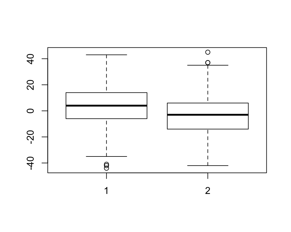
Check the assumptions in R, these are in fact are very common for other tests, including ANOVA and linear model.
Normality To check for normality or in other words, if the variables we want to analyse are normally distributed we can use both specific statistical tests and histograms. Shapiro-Wilk test in R can let you check this in one go, try the following:
#The test
shapiro.test(books$comic)
##
## Shapiro-Wilk normality test
##
## data: books$comic
## W = 0.99677, p-value = 0.421shapiro.test(books$statbook)##
## Shapiro-Wilk normality test
##
## data: books$statbook
## W = 0.99612, p-value = 0.2609# Check visually for normality
par(mfrow=c(2,2)) # par() here displays plots in a 2 by 2 matrix
hist(books$comic, main = "Comic", xlab="Happiness Comic books")
hist(books$statbook, main = "Statbook", xlab= "Happiness Stats books")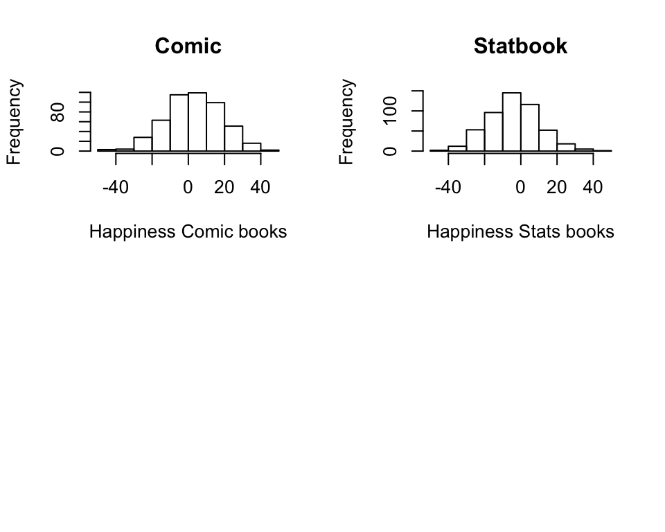
Or using qqnorm:
qqnorm(books$comic, main = "comic")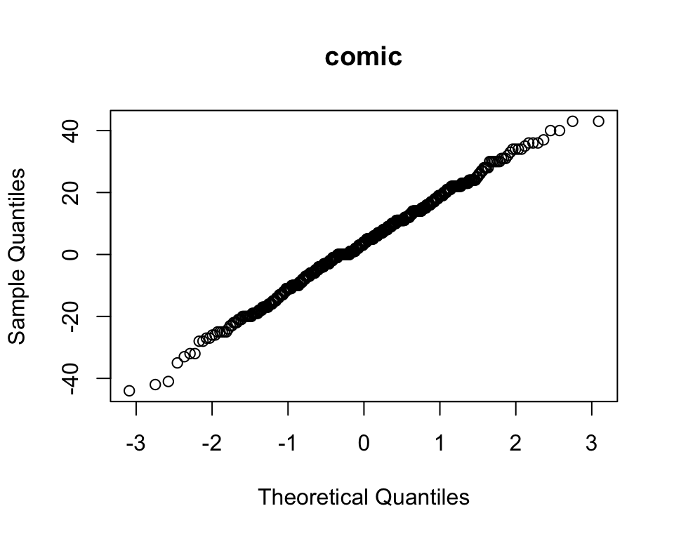
qqnorm(books$statbook, main = "statbook")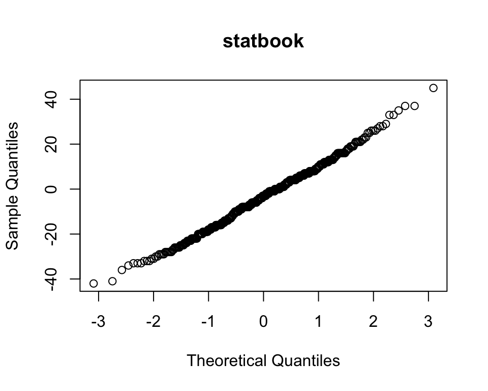
Variance check
To check whether you have an equal variance among two groups we can use a test as well. Conveniently, it is called var.tess and the null hypothesis we are testing is whether the ratio of two variances is equal to one or in other words:
# Check for equality of variance
var.test(books$comic, books$statbook, ratio = 1, conf.level = .95)
##
## F test to compare two variances
##
## data: books$comic and books$statbook
## F = 1.1324, num df = 499, denom df = 499, p-value = 0.1652
## alternative hypothesis: true ratio of variances is not equal to 1
## 95 percent confidence interval:
## 0.949963 1.349898
## sample estimates:
## ratio of variances
## 1.13241Looking good!
Finally lets run the test.*
Examine the arguments below carefully and pick whether you want to use paired or var.equal.
The one we will use:
# Paired t-test
t.test(books$comic, books$statbook, paired = TRUE, var.equal = TRUE)
##
## Paired t-test
##
## data: books$comic and books$statbook
## t = 7.4608, df = 499, p-value = 3.847e-13
## alternative hypothesis: true difference in means is not equal to 0
## 95 percent confidence interval:
## 5.31574 9.11626
## sample estimates:
## mean of the differences
## 7.216Study the results. What do you conclude?
11.2 Chi squared distribution and test
When discussing the uses of the normal distribution we generally assumed a large number of samples (> 30), here we consider small samples (< 30) theory. A more suitable name could be exact sampling theory since the results obtained hold for large samples as well as small samples. Three important small samples distributions are the chi-square distribution, F distribution and the Student’s t-test distribution.
11.2.1 Contingency tables
A categorical variable consists of possible responses in the form of a set of categories rather than numbers on a continuous scale. Categorical variable may be inherently categorical, such as gender male, female or other, or political affiliation. Or they may be created by categorizing a continuous or discrete variable. For example, blood pressure can be recorded in specific measurements such as 120/80 mmHg, or defined as “low”, “normal”, “pre-hypertensive”, “hypertensive”.
Ordinal variables are categorical variables in which the categories might be ranked in order, such as the Likert scale (strongly agree, agree, neutral, disagree and strongly disagree). A specific set of analytical techniques has been developed for ordinal data, even if categorical techniques can also be applied.
11.3 Chi squared distribution
Hypothesis testing on categorical variables requires a way to evaluate whether our results are significant. With RxC tables, the statistic of choice is often one of the chi-square tests, which draw on known properties of the chi-square distribution. Chi-square is sometimes written using the Greek alphabet letter chi to the power of 2: 𝝌𝟐
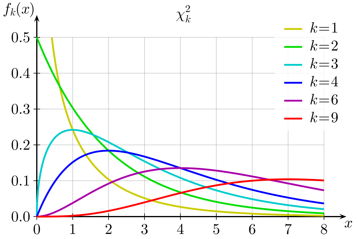
The chi-square distribution is a continuous theoretical probability distribution, a special case of the gamma distribution, with only one parameter k which specifies the degrees of freedom (remember, the normal distribution had two parameters: the mean and the standard deviation). The chi-square distribution only has positive values, because is based on the sum of squared quantities (as indicated by its name, chi square), and is right-skewed. The distribution shape varies according to the value of k. As k approaches infinity, the chi-square distribution approaches a normal distribution.
For this exercise, we can generate the data ourselves. We want to replicate the following table:
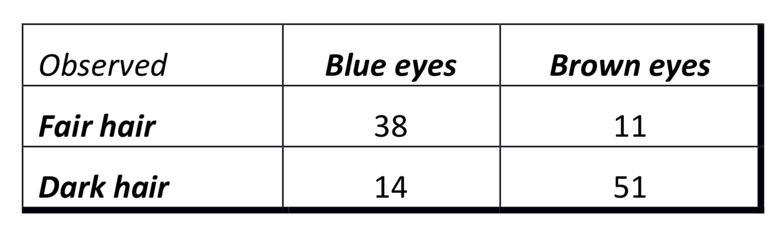
eyedata <- matrix(c(38, 14, 11, 51), nrow = 2)We can then run the test and assign the results to the object (i.e. ‘results’)
results <- chisq.test(eyedata)
results
##
## Pearson's Chi-squared test with Yates' continuity correction
##
## data: eyedata
## X-squared = 33.112, df = 1, p-value = 8.7e-09We can further analyse the residuals. This is one of the approaches to study which cells contributed to significance of the test. A residual is the difference between the observed and expected values for a cell. The larger the residual, the greater the contribution of the cell to the magnitude of the resulting chi-square.
#Get the residuals from the results object
results$residuals
## [,1] [,2]
## [1,] 3.310112 -3.031437
## [2,] -2.873982 2.632024What do you conclude?
11.4 One way Anova example
Here we will present you with a simple one way ANOVA example, we extend on the t test we saw earlier. The extensions to other type of ANOVA in fact can be easily build on top of this baseline. If you are dealing with repeated measures ANOVA, you will find package ezAnova to be quite useful. We wont be covering it here but we hope that once you mastered R over these two days you wont need our help to get yourself going with other packages :)
We will use the data set that has data on effects on blood pressure from taking various pain-relief medication. We will also have one control group.
#Load the data
experiment<-read.csv('dose.csv')
#Recode as factor
experiment$dose <- factor(experiment$dose, levels=c(1,2,3), labels = c("Placebo", "Low_dose", "High_dose"))Lets summarize the data. In R in fact there are quite a few ways that can present you nice descriptive statistics of variables by groups.
Using describe from psych:
describeBy(experiment$effect, experiment$dose)##
## Descriptive statistics by group
## group: Placebo
## vars n mean sd median trimmed mad min max range skew kurtosis se
## X1 1 5 2.2 1.3 2 2.2 1.48 1 4 3 0.26 -1.96 0.58
## --------------------------------------------------------
## group: Low_dose
## vars n mean sd median trimmed mad min max range skew kurtosis se
## X1 1 5 3.2 1.3 3 3.2 1.48 2 5 3 0.26 -1.96 0.58
## --------------------------------------------------------
## group: High_dose
## vars n mean sd median trimmed mad min max range skew kurtosis se
## X1 1 5 5 1.58 5 5 1.48 3 7 4 0 -1.91 0.71#And plot using boxplot directly
boxplot(experiment$effect~ experiment$dose, ylab='Pain Relief Effect',
main='Effect on pain from each condition', col='grey')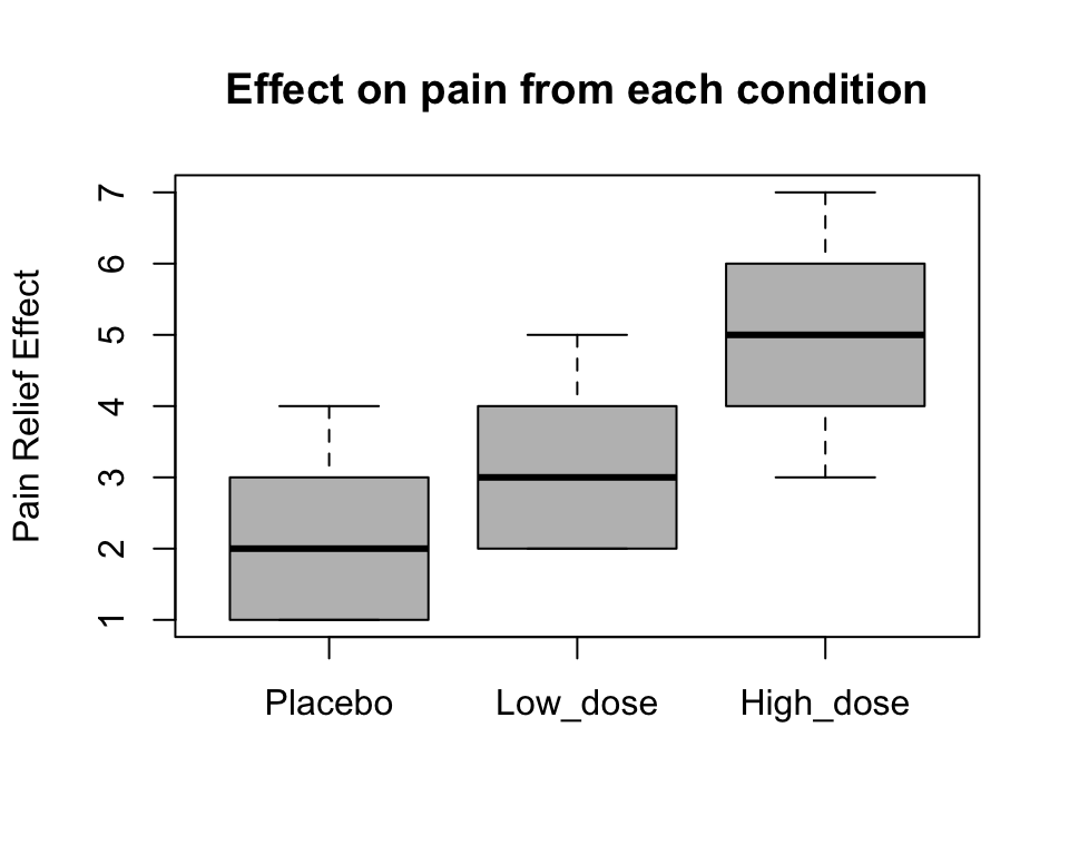
We can also extract the means and sd for our groups:
#Get the means
means <- by(data = experiment[, "effect"], INDICES = experiment$dose, FUN = mean)
means
## experiment$dose: Placebo
## [1] 2.2
## --------------------------------------------------------
## experiment$dose: Low_dose
## [1] 3.2
## --------------------------------------------------------
## experiment$dose: High_dose
## [1] 5#Get standard deviaation
by(data = experiment[, "effect"], INDICES = experiment$dose, FUN = sd)## experiment$dose: Placebo
## [1] 1.30384
## --------------------------------------------------------
## experiment$dose: Low_dose
## [1] 1.30384
## --------------------------------------------------------
## experiment$dose: High_dose
## [1] 1.581139Other way would be to install ’ pasctecs’ and get full descriptives for each group, including confidence intervals and standard error of the mean estimate:
# install 'pasctecs' and get detailed descriptive stats for each group
library(pastecs)
by(data = experiment[, "effect"], INDICES = experiment$dose, FUN = stat.desc)
## experiment$dose: Placebo
## nbr.val nbr.null nbr.na min max
## 5.0000000 0.0000000 0.0000000 1.0000000 4.0000000
## range sum median mean SE.mean
## 3.0000000 11.0000000 2.0000000 2.2000000 0.5830952
## CI.mean.0.95 var std.dev coef.var
## 1.6189318 1.7000000 1.3038405 0.5926548
## --------------------------------------------------------
## experiment$dose: Low_dose
## nbr.val nbr.null nbr.na min max
## 5.0000000 0.0000000 0.0000000 2.0000000 5.0000000
## range sum median mean SE.mean
## 3.0000000 16.0000000 3.0000000 3.2000000 0.5830952
## CI.mean.0.95 var std.dev coef.var
## 1.6189318 1.7000000 1.3038405 0.4074502
## --------------------------------------------------------
## experiment$dose: High_dose
## nbr.val nbr.null nbr.na min max
## 5.0000000 0.0000000 0.0000000 3.0000000 7.0000000
## range sum median mean SE.mean
## 4.0000000 25.0000000 5.0000000 5.0000000 0.7071068
## CI.mean.0.95 var std.dev coef.var
## 1.9632432 2.5000000 1.5811388 0.3162278We can now run ANOVA, but let us first check that the assumption for the equal variances is met:
#Leven test to check for variances being the same, we will need to load package 'car' first
library('car')
Levene test:
leveneTest(y =experiment$effect, group = experiment$dose, center = median)## Levene's Test for Homogeneity of Variance (center = median)
## Df F value Pr(>F)
## group 2 0.1176 0.89
## 12#Run ANOVA
drugAnova <- aov(formula = effect ~ dose, data = experiment)
#Summarise
summary(drugAnova)## Df Sum Sq Mean Sq F value Pr(>F)
## dose 2 20.13 10.067 5.119 0.0247 *
## Residuals 12 23.60 1.967
## ---
## Signif. codes: 0 '***' 0.001 '**' 0.01 '*' 0.05 '.' 0.1 ' ' 1#Summarise as linear model
summary.lm(drugAnova)##
## Call:
## aov(formula = effect ~ dose, data = experiment)
##
## Residuals:
## Min 1Q Median 3Q Max
## -2.0 -1.2 -0.2 0.9 2.0
##
## Coefficients:
## Estimate Std. Error t value Pr(>|t|)
## (Intercept) 2.2000 0.6272 3.508 0.00432 **
## doseLow_dose 1.0000 0.8869 1.127 0.28158
## doseHigh_dose 2.8000 0.8869 3.157 0.00827 **
## ---
## Signif. codes: 0 '***' 0.001 '**' 0.01 '*' 0.05 '.' 0.1 ' ' 1
##
## Residual standard error: 1.402 on 12 degrees of freedom
## Multiple R-squared: 0.4604, Adjusted R-squared: 0.3704
## F-statistic: 5.119 on 2 and 12 DF, p-value: 0.02469So what do we conclude? You can see that ANOVA results only can suggest that there were some differences across three groups but we still know nothing about which group was different. Linear regression may aid our understanding about which means was significantly different/more specifically we can see how much difference in expected effect on pain relief can be found from high and low dose of medicine versus the placebo.