Chapter 3 Basic principles of R programming
3.1 If you want to keep it, put it in a box
Everything in life is merely transient; we ourselves are pretty ephemeral beings. (#sodeepbro) However, R takes this quality and runs with it. If you ask R to perform any operation, it will spew it out into the console and immediately forget it ever happened. Let’s show you what that means:
# create an object a and assign it the value of 1
a <- 1

# increment a by 1
a + 1
## [1] 2# OK, now see what the value of a is
a## [1] 1
So, R as if forgot we asked it to do a + 1 and didn’t change its value. The only way to keep this new value is to put it in an object.
b <- a + 1

# now let's see
b
## [1] 2
Think of objects as boxes. The names of the objects are only labels. Just like with boxes, it is convenient to label boxes in a way that is indicative of their contents, but the label itself does not determine the content. Sure, you can create an R object called one and store the value of 2 in it, if you wish. But you might want to think about whether or not it is a helpful name. And what kind of person that makes you… Objects can contain anything at all: values, vectors, matrices, data, graphs, tables, even code. In fact, every time you call a function, e.g., mean(), you are running the code that’s inside the object mean with whatever values you pass to the arguments of the function.
Let’s demonstrate this last point:
# let's create a vector of numbers the mean of which I want to calculate
vec <- c(103, 1, 1, 6, 3, 43, 2, 23, 7, 1)

# see what's inside
vec
## [1] 103 1 1 6 3 43 2 23 7 1# let's get the mean
# mean is the sum of all values divided by the number of values
sum(vec)/length(vec)## [1] 19# good, now let's create a function that calculates
# the mean of whatever we ask it to
function(x) {sum(x)/length(x)}## function(x) {sum(x)/length(x)}
## <environment: 0x7f9082ff2bc0># but as we discussed above, R immediately forgot about the function
# so we need to store it in a box (object) to keep it for later!
calc.mean <- function(x) {sum(x)/length(x)}
# OK, all ready now
calc.mean(x = vec)## [1] 19# the code inside the object calc.mean is reusable
calc.mean(x = c(3, 5, 53, 111))## [1] 43# to show that calc.mean is just an object with some code in it,
# you can look inside, just like with any other object
calc.mean## function(x) {sum(x)/length(x)}
## <environment: 0x7f9082ff2bc0>
Let this be your mantra: “If I want to keep it for later, I need to put it in an object so that is doesn’t go off.”
3.2 You can’t really change an object
Unlike in the physical world, objects in R cannot truly change. The reason is that, sticking to our analogy, these objects are kind of like boxes. You can put stuff in, take stuff out and that’s pretty much it. However, unlike boxes, when you take stuff out of objects, you only take out a copy of its contents. The original contents of the box remain intact. Of course you can do whatever you want (within limits) to the stuff once you’ve taken it out of the box but you are only modifying the copy. And unless you put that modified stuff into a box, R will forget about it as soon as it’s done with it. Now, as you probably know, you can call the boxes whatever you want (again, within certain limits). What might not have occurred to you though, is that you can call the new box the same as the old one. When that happens, R basically takes the label off the old box, pastes it on the new one and burns the old box. So even though some operations in R may look like they change objects, under the hood R copies their content, modifies it, stores the result in a different object puts the same label on it and discards the original object. Understanding this mechanism will make things much easier!
Putting the above into practice, this is how you “change” an R object:
# put 1 into an object (box) called a
a <- 1

# copy the content of a, add 1 to it and store it in an object b
b <- a + 1

# copy what's inside b and put it in a new object called a
# discarding the old object a
a <- b

# now see what's inside of a
# (by copying its content and pasting it in the console)
a
## [1] 2
Of course, you can just cut out the middleman (object b). So to increment a by another 1, we can do:
a <- a + 1

a
## [1] 3
3.3 It’s elementary, my dear Watson
When it comes to data, every vector, matrix, list, data frame - in other words, every structure - is composed of elements. An element is a single number, boolean (TRUE/FALSE), or a character string (anything in “quotes”). Elements come in several classes:
"numeric", as the name suggests, a numeric element is a single number: 1, 2, -725, 3.14159265, etc.. A numeric element is never in ‘single’ or “double” quotes! Numbers are cool because you can do a lot of maths (and stats!) with them."character", a string of characters, no matter how long. It can be a single letter,'g', but it can equally well be a sentence,"Elen s?la lumenn' omentielvo."(if you want the string to contain any single quotes, use double quotes to surround the string with and vice versa). Notice that character strings inRare always in ‘single’ or “double” quotes. Conversely anything in quotes is a character string:class(3)## [1] "numeric"class("3") # in quotes, therefore character!## [1] "character"It stands to reason that you can’t do any maths with cahracter strings, not even if it’s a number that’s inside the quotes!
"3" + "2"## Error in "3" + "2": non-numeric argument to binary operator"logical", a logical element can take one of two values,TRUEorFALSE. Logicals are usually the output of logical operations (anything that can be phrased as a yes/no question, e.g., is x equal to y?). In formal logic,TRUEis represented as 1 andFALSEas 0. This is also the case inR:# recall that c() is used to bind elements into a vector # (that's just a fancy term for an ordered group of elements) class(c(TRUE, FALSE))## [1] "logical"# we can force ('coerce', in R jargon) the vector to be numeric as.numeric(c(TRUE, FALSE))## [1] 1 0This has interesting implications. First, is you have a logical vector of many
TRUEs andFALSEs, you can quickly count the number ofTRUEs by just taking the sum of the vector:# consider vector of 50 logicals x## [1] FALSE TRUE TRUE TRUE FALSE FALSE TRUE TRUE TRUE FALSE TRUE ## [12] TRUE TRUE FALSE TRUE TRUE TRUE TRUE TRUE FALSE TRUE TRUE ## [23] FALSE TRUE TRUE TRUE TRUE TRUE TRUE FALSE TRUE TRUE TRUE ## [34] FALSE FALSE FALSE TRUE TRUE TRUE TRUE TRUE TRUE TRUE TRUE ## [45] TRUE TRUE FALSE TRUE TRUE TRUE# number of TRUEs sum(x)## [1] 38# number of FALSEs is 50 minus number of TRUEs length(x) - sum(x)## [1] 12Second, you can perform all sorts of arithmetic operations on logicals:
# TRUE/FALSE can be shortened to T/F
T + T
## [1] 2F - T## [1] -1(T * T) + F## [1] 1Third, you can coerce numeric elements to valid logicals:
# zero is FALSE
as.logical(0)
## [1] FALSE# everything else is TRUE as.logical(c(-1, 1, 12, -231.3525))## [1] TRUE TRUE TRUE TRUENow, you may wonder that use this can possible be?! Well, this way you can perform basic logical operations, such as AND, OR, and XOR (see section “Handy functions that return logicals” below):
# x * y is equivalent to x AND y
as.logical(T * T)
## [1] TRUEas.logical(T * F)## [1] FALSEas.logical(F * T)## [1] FALSEas.logical(F * F)## [1] FALSE# x + y is equivalent to x OR y as.logical(T + T)## [1] TRUEas.logical(T + F)## [1] TRUEas.logical(F + T)## [1] TRUEas.logical(F + F)## [1] FALSE# x - y is equivalent to x XOR y (eXclusive OR, either-or) as.logical(T - T)## [1] FALSEas.logical(T - F)## [1] TRUEas.logical(F - T)## [1] TRUEas.logical(F - F)## [1] FALSE"factor", factors are a bit weird. They are used mainly for tellingRthat a vector represents a categorical variable. For instance, you can be comparing two groups, treatment and control.# create a vector of 15 "control"s and 15 "treatment"s # rep stands for 'repeat', which is exactly what the function does x <- rep(c("control", "treatment"), each = 15) x## [1] "control" "control" "control" "control" "control" ## [6] "control" "control" "control" "control" "control" ## [11] "control" "control" "control" "control" "control" ## [16] "treatment" "treatment" "treatment" "treatment" "treatment" ## [21] "treatment" "treatment" "treatment" "treatment" "treatment" ## [26] "treatment" "treatment" "treatment" "treatment" "treatment"# turn x into a factor x <- as.factor(x) x## [1] control control control control control control control ## [8] control control control control control control control ## [15] control treatment treatment treatment treatment treatment treatment ## [22] treatment treatment treatment treatment treatment treatment treatment ## [29] treatment treatment ## Levels: control treatmentThe first thing to notice is the line under the last printout that says “
Levels: control treatment”. This informs you thatxis now a factor with two levels (or, a categorical variable with two categories).Second thing you should take note of is that the words
controlandtreatmentdon’t have quotes around them. This is another wayRuses to tell you this is a factor.With factors, it is important to understand how they are represented in
R. Despite, what they look like, under the hood, they are numbers. A one-level factor is a vector of1s, a two-level factor is a vector of1s and2s, a n-level factor is a vector of1s,2s,3s … ns. The levels, in our casecontrolandtreatment, are just labels attached to the1s and2s. Let’s demonstrate this:typeof(x)## [1] "integer"# integer is fancy for "whole number" # we can coerce factors to numeric, thus stripping the labels as.numeric(x)## [1] 1 1 1 1 1 1 1 1 1 1 1 1 1 1 1 2 2 2 2 2 2 2 2 2 2 2 2 2 2 2# see the labels levels(x)## [1] "control" "treatment"The labels attached to the numbers in a factor can be whatever. Let’s say that in your raw data file, treatment group is coded as 1 and control group is coded as 0.
# create a vector of 15 zeros and 15 ones
x <- rep(0:1, each = 15)
x
## [1] 0 0 0 0 0 0 0 0 0 0 0 0 0 0 0 1 1 1 1 1 1 1 1 1 1 1 1 1 1 1# turn x into a factor x <- as.factor(x) x## [1] 0 0 0 0 0 0 0 0 0 0 0 0 0 0 0 1 1 1 1 1 1 1 1 1 1 1 1 1 1 1 ## Levels: 0 1Since
xis now a factor with levels0and1, we know that it is stored inRas a vector of1s and2s and the zeros and ones, representing the groups, are only labels:as.numeric(x)## [1] 1 1 1 1 1 1 1 1 1 1 1 1 1 1 1 2 2 2 2 2 2 2 2 2 2 2 2 2 2 2levels(x)## [1] "0" "1"The fact that factors in
Rare represented as labelled integers has interesting implications some of you have already come across. First, certain functions will coerce factors into numeric vectors which can shake things up. This happened when you usedcbind()on a factor with levels0and1:x## [1] 0 0 0 0 0 0 0 0 0 0 0 0 0 0 0 1 1 1 1 1 1 1 1 1 1 1 1 1 1 1 ## Levels: 0 1# let's bind the first 15 elements and the last 15 elements together as columnscbind(x[1:15], x[16:30])## [,1] [,2] ## [1,] 1 2 ## [2,] 1 2 ## [3,] 1 2 ## [4,] 1 2 ## [5,] 1 2 ## [ reached getOption("max.print") -- omitted 10 rows ]# printout truncated to first 5 rows to save spacecbind()binds the vectors you provide into the columns of a matrix. Since matrices (yep, that’s the plural of ‘matrix’; also, more on matrices later) can only containlogical,numeric, andcharacterelements, thecbind()function coerces the elements of thexfactor (haha, the X-factor) intonumeric, stripping the labels and leaving only1s and2s.The other two consequences of this labelled numbers system stem from the way the labels are stored. Every
Robject comes with a list of so called attributes attached to it. These are basically information about the object. For objects of classfactor, the attributes include its levels (or the labels attached to the numbers) and class:attributes(x)## $levels ## [1] "0" "1" ## ## $class ## [1] "factor"So the labels are stored separately of the actual elements. This means, that even if you delete some of the numbers, the labels stay the same. Let’s demonstrate this implication on the
plot()function. This function is smart enough to know that if you give it a factor it should plot it using a bar chart, and not a histogram or a scatter plot:plot(x)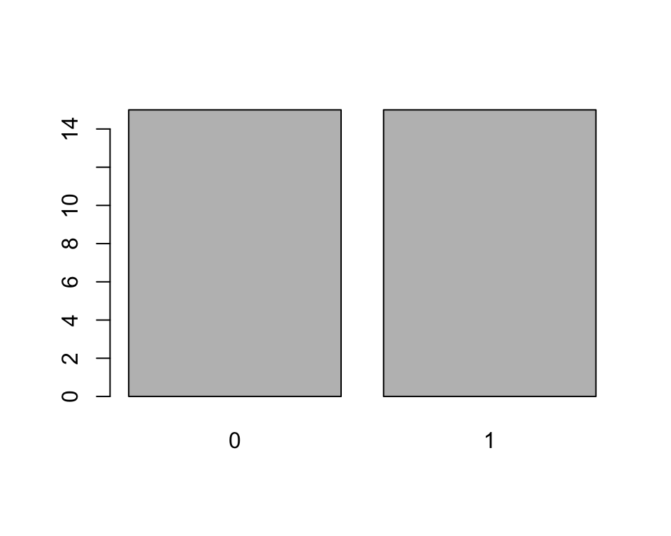
Now, let’s take the first 15 elements of
x, which are all0s and plot them:y <- x[1:15] y## [1] 0 0 0 0 0 0 0 0 0 0 0 0 0 0 0 ## Levels: 0 1plot(y)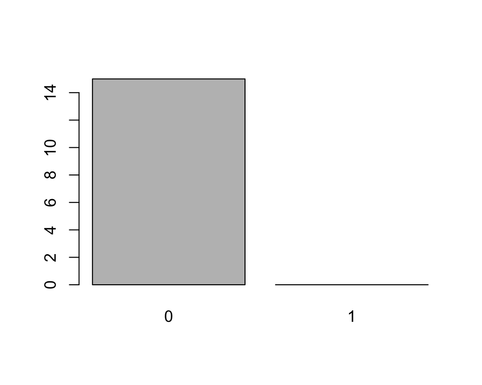
Even though our new object
yonly includes0s, thelevelsattribute still tellsRthat this is a factor of (at least potentially) two levels:"0"and"1"and soplot()leaves a room for the1s.The last consequence is directly related to this. Since the levels of an object of class
factorare stored as its attributes, any additional values put inside the objects will be invalid and turned intoNAs (Rwill warn us of this). In other words, you can only add those values that are among the ones produced bylevels()to an object of classfactor:# try adding invalid values -4 and 3 to the end of vector x x[31:32] <- c(-4, 3)## Warning in `[<-.factor`(`*tmp*`, 31:32, value = c(-4, 3)): invalid factor ## level, NA generatedx## [1] 0 0 0 0 0 0 0 0 0 0 0 0 0 0 ## [15] 0 1 1 1 1 1 1 1 1 1 1 1 1 1 ## [29] 1 1 <NA> <NA> ## Levels: 0 1The only way to add these values to a factor is to first coerce it to
numeric, then add the values, and then turn it back intofactor:# coerce x to numeric x <- as.numeric(x[1:30]) class(x)## [1] "numeric"# but remember that 0s and 1s are now 1s and 2s! x## [1] 1 1 1 1 1 1 1 1 1 1 1 1 1 1 1 2 2 2 2 2 2 2 2 2 2 2 2 2 2 2# so subtract 1 to make the values 0s and 1s again x <- x - 1 # add the new values x <- c(x, -4, 3) # back into fractor x <- as.factor(x) x## [1] 0 0 0 0 0 0 0 0 0 0 0 0 0 0 0 1 1 1 1 1 1 1 1 ## [24] 1 1 1 1 1 1 1 -4 3 ## Levels: -4 0 1 3# SUCCESS! # reset x <- as.factor(rep(0:1, each = 15)) # one-liner x <- as.factor(c(as.numeric(x[1:30]) - 1, -4, 3)) x## [1] 0 0 0 0 0 0 0 0 0 0 0 0 0 0 0 1 1 1 1 1 1 1 1 ## [24] 1 1 1 1 1 1 1 -4 3 ## Levels: -4 0 1 3Told you factors were weird…
"ordered", finally, these are the same as factors but, in addition to having levels, these levels are ordered and thus allow comparison (notice theLevels: 0 < 1below):# coerce x to numeric x <- as.ordered(rep(0:1, each = 15)) x## [1] 0 0 0 0 0 0 0 0 0 0 0 0 0 0 0 1 1 1 1 1 1 1 1 1 1 1 1 1 1 1 ## Levels: 0 < 1# we can now compare the levels x[1] < x[30]## [1] TRUE# this is not the case with factors y <- as.factor(rep(0:1, each = 15)) y[1] < y[30]## Warning in Ops.factor(y[1], y[30]): '<' not meaningful for factors## [1] NAObjects of class
orderedare useful for storing ordinal variables, e.g., age group.
In addition to these five sorts of elements, there are three special wee snowflakes:
NA, stands for “not applicable” and is used for missing data. Unlike other kinds of elements, it can be bound into a vector along with elements of any class.NaN, stands for “not a number”. It is technically of classnumericbut only occurs as the output of invalid mathematical operations, such as dividing zero by zero or taking a square root of a negative number:0 / 0## [1] NaNsqrt(-12)## Warning in sqrt(-12): NaNs produced## [1] NaNInf(or-Inf), infinity. Reserved for division of a non-zero number by zero (no, it’s not technically right):235/0## [1] Inf-85.123/0## [1] -Inf
3.3.1 Data structures
So that’s most of what you need to know about elements. Let’s talk about putting elements together. As mentioned above, elements can be grouped in various data structures. These differ in the ways in which they arrange elements:
vectors arrange elements in a line. they don’t have dimensions and can only contain elements of same class (e.g.,
"numeric","character","logical").# a vector letters[5:15]## [1] "e" "f" "g" "h" "i" "j" "k" "l" "m" "n" "o"If you try to force elements of different classes to a single vector, they will all be converted to the most complex class. The order of complexity, from least to most complex, is:
logical,numeric, andcharacter. Elements of classfactorandorderedcannot be meaningfully bound in a vector with other classes (nor with each other): they either get converted tonumeric,character- if you’re lucky - or toNA.# c(logical, numeric) results in numeric x <- c(T, F, 1:6) x## [1] 1 0 1 2 3 4 5 6class(x)## [1] "integer"# integer is like numeric but only for whole numbers to save computer memory # adding character results in character x <- c(x, "foo") # the numbers 1-6 are not numeric any more! x## [1] "1" "0" "1" "2" "3" "4" "5" "6" "foo"class(x)## [1] "character"matrices arrange elements in a square/rectangle, i.e., a two-dimensional arrangement of rows and columns. They can also only accommodate elements of the same class and cannot store attributes of elements. That means, you can’t use them to store (ordered) factors.
# a matrix
matrix(rnorm(20, 1, 1), ncol = 5) # must be square/rectangular
## [,1] [,2] [,3] [,4] [,5] ## [1,] 0.7655198 1.2890311 1.6610137 1.246979 -0.390655572 ## [2,] 1.9004878 0.5683308 0.6289706 1.036021 0.671293584 ## [3,] -0.6435008 -0.4605371 1.4222572 1.158418 1.687722062 ## [4,] -2.0320610 -0.5412433 2.5493071 1.735854 -0.004761932# not suitable for factors x <- factor(rbinom(10, 1, .5)) x## [1] 1 1 1 0 0 0 1 1 1 1 ## Levels: 0 1# not factors any more! matrix(x, ncol = 5)## [,1] [,2] [,3] [,4] [,5] ## [1,] "1" "1" "0" "1" "1" ## [2,] "1" "0" "0" "1" "1"lists arrange elements in a collection of vectors or other data structures. Different vectors/structures can be of different lengths and contain elements of different classes. Elements of lists and, by extension, data frames can be accessed using the
$operator, provided we gave them names.# a list my_list <- list( # 1st element of list is a numeric matrix A = matrix(rnorm(20, 1, 1), ncol = 5), # 2nd element is a character vector B = letters[1:5], # third is a data.frame C = data.frame(x = c(1:3), y = LETTERS[1:3]) ) my_list## $A ## [,1] [,2] [,3] [,4] [,5] ## [1,] 0.7759403 -0.4469245 0.2663765 1.2538539 0.9723083 ## [2,] 0.2519247 0.4254006 2.4120504 -0.3848255 2.1041691 ## [3,] 0.2322069 1.6991658 -0.3048592 1.3873206 1.6660872 ## [4,] 0.3102466 1.6090666 -0.7088821 1.4769681 1.0728583 ## ## $B ## [1] "a" "b" "c" "d" "e" ## ## $C ## x y ## 1 1 A ## 2 2 B ## 3 3 C# we can use the $ operator to access NAMED elements of lists my_list$B## [1] "a" "b" "c" "d" "e"# this is also true for data frames my_list$C$x## [1] 1 2 3# but not for vectors or matrices my_list$A$1## Error: <text>:2:11: unexpected numeric constant ## 1: # but not for vectors or matrices ## 2: my_list$A$1 ## ^data frames are lists but have an additional constraint: all the vectors of a
data.framemust be of the same length. That is the reasons why your datasets are always rectangular.
Different data structures are useful for different things but bear in mind that, ultimately, they are all just bunches of elements. This understanding is crucial for working with data.
3.4 There are only three ways to ask for elements
Now that you understand that all data boil down to elements, let’s look at how to ask R for the elements you want.
As the section heading suggests, there are only three ways to do this:
- indices
- logical vector
- names (only if elements are named, usually in lists and data frames)
Let’s take a closer look at these ways one at a time.
3.4.1 Indices
The first way to ask for an element is to simply provide the numeric position of the desired element in the structure (vector, list…) in a set of square brackets [] at the end of the object name:
x <- c("I", " ", "l", "o", "v", "e", " ", "R")

# get the 6th element
x[6]
## [1] "e"
To get more than just one element at a time, you need to provide a vector of indices. For instance, to get the elements 3-6 of x, we can do:
x[3:6]## [1] "l" "o" "v" "e"# equivalent to
x[c(3, 4, 5, 6)]## [1] "l" "o" "v" "e"
Remember that some structures can contain as their elements other structures. For example asking for the first element of my_list will return:
my_list[1]## $A
##           [,1]       [,2]       [,3]       [,4]      [,5]
## [1,] 0.7759403 -0.4469245  0.2663765  1.2538539 0.9723083
## [2,] 0.2519247  0.4254006  2.4120504 -0.3848255 2.1041691
## [3,] 0.2322069  1.6991658 -0.3048592  1.3873206 1.6660872
## [4,] 0.3102466  1.6090666 -0.7088821  1.4769681 1.0728583
The $A at the top of the output indicates that we have accessed the element A of my_list but not really accessed the matrix itself. Thus, at this stage, we wouldn’t be able to ask for its elements. To access the matrix contained in my_list$A, we need to write either exactly that, or use double brackets:
my_list[[1]]## [,1] [,2] [,3] [,4] [,5]
## [1,] 0.7759403 -0.4469245 0.2663765 1.2538539 0.9723083
## [2,] 0.2519247 0.4254006 2.4120504 -0.3848255 2.1041691
## [3,] 0.2322069 1.6991658 -0.3048592 1.3873206 1.6660872
## [4,] 0.3102466 1.6090666 -0.7088821 1.4769681 1.0728583# with the $A now gone from output, we can access the matrix itself
my_list[[1]][1]## [1] 0.7759403
As discussed above, some data structures are dimensionless (vectors, lists), while others are arranged in n-dimensional rectangles (where n > 1). When indexing/subsetting elements of dimensional structures, we need to provide coordinates of the elements for each dimension. This is done by providing n numbers or vectors in the []s separated by a comma.
A matrix, for instance has 2 dimensions, rows and columns. The first number/vector in the []s represents rows and the second columns. Leaving either position blank will return all rows/columns:
mat <- matrix(LETTERS[1:20], ncol = 5)
mat
## [,1] [,2] [,3] [,4] [,5]
## [1,] "A" "E" "I" "M" "Q"
## [2,] "B" "F" "J" "N" "R"
## [3,] "C" "G" "K" "O" "S"
## [4,] "D" "H" "L" "P" "T"# blank spaces technically not needed but improve code readability
mat[1, ] # first row## [1] "A" "E" "I" "M" "Q"mat[ , 1] # first column## [1] "A" "B" "C" "D"mat[c(2, 4), ] # rows 2 and 4, notice the c()## [,1] [,2] [,3] [,4] [,5]
## [1,] "B" "F" "J" "N" "R"
## [2,] "D" "H" "L" "P" "T"mat[c(2, 4), 1:3] # elements 2 and 4 of columns 1-3## [,1] [,2] [,3]
## [1,] "B" "F" "J"
## [2,] "D" "H" "L"
To get the full matrix, we simply type its name. However, you can think of the same operation as asking for all rows and all columns of the matrix:
mat[ , ] # all rows, all columns## [,1] [,2] [,3] [,4] [,5]
## [1,] "A" "E" "I" "M" "Q"
## [2,] "B" "F" "J" "N" "R"
## [3,] "C" "G" "K" "O" "S"
## [4,] "D" "H" "L" "P" "T"
The same is the case with data frames:
df <- data.frame(id = LETTERS[1:6],
                group = rep(c("Control", "Treatment"), each = 3),
                score = rnorm(6, 100, 20))
df
## id group score
## 1 A Control 101.99636
## 2 B Control 100.49968
## 3 C Control 101.22448
## 4 D Treatment 115.57397
## 5 E Treatment 107.48837
## 6 F Treatment 74.64442df[1, ] # first row## id group score
## 1 A Control 101.9964df[4:6, c(1, 3)]## id score
## 4 D 115.57397
## 5 E 107.48837
## 6 F 74.64442
Take home message: when using indices to ask for elements, remember that to request more than one, you need to give a vector of indices (i.e., numbers bound in a c()). Also remember that some data structures need you to specify dimensions separated by a comma (most often just rows and columns for matrices and data frames).
3.4.2 Logical vectors
The second way of asking for elements is by putting a vector of logical (AKA Boolean) values in the []s. An important requirement here is that the vector must be the same length as the one being subsetted. So, for a vector with three elements, we need to provide three logical values, TRUE for “I want this one” and FALSE for “I don’t want this one”. Let’s demonstrate this on the same vector we used for indices:
x <- c("I", " ", "l", "o", "v", "e", " ", "R")

# get the 6th element
x[c(F, F, F, F, F, T, F, F)]
## [1] "e"#get elements 3-6
x[c(F, F, T, T, T, T, F, F)]## [1] "l" "o" "v" "e"
All the other principles we talked about regarding indexing apply also to logical vectors. Note also, that higher 2D structures need a logical row vector and a logical column vector:
# recall our mat
mat
## [,1] [,2] [,3] [,4] [,5]
## [1,] "A" "E" "I" "M" "Q"
## [2,] "B" "F" "J" "N" "R"
## [3,] "C" "G" "K" "O" "S"
## [4,] "D" "H" "L" "P" "T"# rows 2 and 4
mat[c(T, F, T, F), ]## [,1] [,2] [,3] [,4] [,5]
## [1,] "A" "E" "I" "M" "Q"
## [2,] "C" "G" "K" "O" "S"# element 4 of rows 1 and 2
mat[c(F, F, F, T), c(T, T, F, F, F)]## [1] "D" "H"# you can even COMBINE the two ways!
mat[4, c(T, T, F, F, F)]## [1] "D" "H"
And as if vectors weren’t enough, you can even use matrices of logical values to subset matrices and data frames:
mat_logic <- matrix(c(rep(c(F, T), each = 3), rep(F, 9), c(T, T, T)), ncol = 3)
mat_logic
## [,1] [,2] [,3]
## [1,] FALSE FALSE FALSE
## [2,] FALSE FALSE FALSE
## [3,] FALSE FALSE FALSE
## [4,] TRUE FALSE TRUE
## [5,] TRUE FALSE TRUE
## [6,] TRUE FALSE TRUEdf[mat_logic]## [1] "D" "E" "F" "115.57397" "107.48837" " 74.64442"
Notice, however, that the output is a vector so two things happened: first, the rectangular structure has been erased and second, since vectors can only contain elements of the same class (see above), the numbers got converted into character strings (hence the ""s). Nevertheless, this method of subsetting using logical matrices can be useful for replacing several values in different rows and columns with another value:
# replace with NAs
df[mat_logic] <- NA
df
## id group score
## 1 A Control 101.9964
## 2 B Control 100.4997
## 3 C Control 101.2245
## 4 <NA> Treatment NA
## 5 <NA> Treatment NA
## 6 <NA> Treatment NA
To use a different example, take the function lower.tri(). It can be used to subset a matrix in order to get the lower triangle (with or without the diagonal). Consider matrix mat2 which has "L"s in its lower triangle, "U"s in its upper triangle, and "D"s on the diagonal:
##      [,1] [,2] [,3] [,4]
## [1,] "D"  "U"  "U"  "U"
## [2,] "L"  "D"  "U"  "U"
## [3,] "L"  "L"  "D"  "U"
## [4,] "L"  "L"  "L"  "D"
Let’s use lower.tri() to ask for the elements in its lower triangle:
mat2[lower.tri(mat2)]## [1] "L" "L" "L" "L" "L" "L"# we got only "L"s, good!
Adding the , diag = T will return the lower triangle along with the diagonal:
mat2[lower.tri(mat2, diag = T)]## [1] "D" "L" "L" "L" "D" "L" "L" "D" "L" "D"# we got only "L"s and "D"s
So what does the function actually do? What is this sorcery? Let’s look at the output of the function:
lower.tri(mat2)## [,1] [,2] [,3] [,4]
## [1,] FALSE FALSE FALSE FALSE
## [2,] TRUE FALSE FALSE FALSE
## [3,] TRUE TRUE FALSE FALSE
## [4,] TRUE TRUE TRUE FALSESo the function produces a matrix of logicals, the same size as out mat2, with TRUEs in the lower triangle and FALSEs elsewhere. What we did above is simply use this matrix to subset mat2[].
If you’re curious how the function produces the logical matrix then, first of all, that’s great, keep it up and second, you can look at the code wrapped in the lower.tri object (since functions are only objects of a special kind with code inside instead of data):
lower.tri

function (x, diag = FALSE)
{
    x <- as.matrix(x)
    if (diag)
        row(x) >= col(x)
    else row(x) > col(x)
}
<bytecode: 0x0000000015a39ab0>
<environment: namespace:base>
Right, let’s see. If we set the diag argument to TRUE the function returns row(x) >= col(x). If we leave it set to FALSE (default), it returns row(x) > col(x). Let’s substitute x for our mat2 and try it out:
row(mat2)## [,1] [,2] [,3] [,4]
## [1,] 1 1 1 1
## [2,] 2 2 2 2
## [3,] 3 3 3 3
## [4,] 4 4 4 4col(mat2)## [,1] [,2] [,3] [,4]
## [1,] 1 2 3 4
## [2,] 1 2 3 4
## [3,] 1 2 3 4
## [4,] 1 2 3 4# diag = TRUE case
row(mat2) >= col(mat2)## [,1] [,2] [,3] [,4]
## [1,] TRUE FALSE FALSE FALSE
## [2,] TRUE TRUE FALSE FALSE
## [3,] TRUE TRUE TRUE FALSE
## [4,] TRUE TRUE TRUE TRUE# use it for subsetting mat2
mat2[row(mat2) >= col(mat2)]## [1] "D" "L" "L" "L" "D" "L" "L" "D" "L" "D"# diag = FALSE case
row(mat2) > col(mat2)## [,1] [,2] [,3] [,4]
## [1,] FALSE FALSE FALSE FALSE
## [2,] TRUE FALSE FALSE FALSE
## [3,] TRUE TRUE FALSE FALSE
## [4,] TRUE TRUE TRUE FALSEmat2[row(mat2) > col(mat2)]## [1] "L" "L" "L" "L" "L" "L"
MAGIC!
Take home message: When subsetting using logical vectors, the vectors must be the same length as the vectors you are subsetting. The same goes for logical matrices: they must be the same size as the matrix/data frame you are subsetting.
3.4.3 Complementary subsetting
Both of the aforementioned ways of asking for subsets of data can be inverted. For indices, you can simply put a - sign before the vector:
# elements 3-6 of x
x[3:6]
## [1] "l" "o" "v" "e"# invert the selection
x[-(3:6)]## [1] "I" " " " " "R"#equivalent to
x[c(1, 2, 7, 8)]## [1] "I" " " " " "R"
For logical subsetting, you need to negate the values. That is done using the logical negation operator ‘!’ (AKA “not”):
y <- T
y
## [1] TRUE# negation
!y## [1] FALSE# also works for vectors and matrices
mat_logic## [,1] [,2] [,3]
## [1,] FALSE FALSE FALSE
## [2,] FALSE FALSE FALSE
## [3,] FALSE FALSE FALSE
## [4,] TRUE FALSE TRUE
## [5,] TRUE FALSE TRUE
## [6,] TRUE FALSE TRUE!mat_logic## [,1] [,2] [,3]
## [1,] TRUE TRUE TRUE
## [2,] TRUE TRUE TRUE
## [3,] TRUE TRUE TRUE
## [4,] FALSE TRUE FALSE
## [5,] FALSE TRUE FALSE
## [6,] FALSE TRUE FALSEdf[!mat_logic]## [1] "A" "B" "C" "Control" "Control"
## [6] "Control" "Treatment" "Treatment" "Treatment" "101.9964"
## [11] "100.4997" "101.2245"
3.4.4 Names - $ subsetting
We already mentioned the final way of subsetting elements when we talked about lists and data frames. To subset top-level elements of a named list or columns of a data frame, we can use the $ operator.
df$group## [1] Control Control Control Treatment Treatment Treatment
## Levels: Control TreatmentWhat we get is a single vector that can be further subsetted using indices or logical vectors:
df$group[c(3, 5)]## [1] Control Treatment
## Levels: Control Treatment
Bear in mind that all data cleaning and transforming ultimately boils down to using one, two, or all of these three ways of subsetting elements!
3.5 Think of commands in terms of their output
In order to be able to manipulate your data, you need to understand that any chunk of code is just a formal representation of what the code is supposed to be doing, i.e., its output. That means that you are free to put code inside []s but only so long as the output of the code is either a numeric vector (of valid values - you cannot ask for x[c(3, 6, 7)] if x has only six elements) or a logical vector/matrix of the same length/size as the object that is being subsetted. Put any other code inside []s and R will return an error (or even worse, quietly produce some unexpected behaviour)!
So the final point we would like to stress is that you need to…
3.6 Know what to expect
You should not be surprised by the outcome of R. If you are, that means you do not entirely understand what you asked R to do. A good way to practice this understanding is to tell yourself what form of output and what values you expect a command to return.
For instance, in the code above, we did x[-(3:6)]. Ask yourself what does the -(3:6) return. How and why is it different from -3:6? What will happen if you do x[-3:6]?
-(3:6)## [1] -3 -4 -5 -6-3:6## [1] -3 -2 -1 0 1 2 3 4 5 6x[-3:6]## Error in x[-3:6]: only 0's may be mixed with negative subscriptsIf any of the output above surprised you, try to understand why. What were your expectations? Do you now, having seen the actual output, understand what those commands do?
Some of you were wondering why, when replacing values in column 1 of matrix mat that are larger than, say, 2 with NAs, you had to specify the column several times, e.g.:
mat[mat[ , 1] > 2, 1] <- NA

## 2 instances of mat[ , 1] in total:
# 1. outer
mat[..., 1]
# 2. comparison
mat[ , 1] > ...
Let’s consider matrix mat:
##            [,1]       [,2]        [,3]        [,4]        [,5]        [,6]
## [1,]  1.5130103  0.9952683 -0.95794125  0.33504342  0.07712739 -0.66372770
## [2,] -0.4376715 -0.2812407 -0.17243454  0.70031135 -0.25902516 -0.09343669
## [3,]  2.4322500 -0.3920698 -0.77261606 -1.28996693  1.03975751  0.15565290
## [4,]  1.7789861 -0.2317490 -0.21926087  0.89101639 -0.52515474  1.43493359
## [5,] -0.8248379  0.7080644 -0.02591484  0.04974556  0.13429166  0.19358823
and think of the command in terms of the expected outcome of its constituent elements. The logical operator ‘>’ returns a logical vector corresponding to the answer to the question “is the value to the left of the operator larger than that to the right of the operator?” The answer can only be TRUE or FALSE. So mat[ , 1] > 2 will return:
## [1] FALSE FALSE TRUE FALSE FALSEThere is no way of knowing that these values correspond to the 1st column of mat just from the output alone. That information has been lost.
This means that, if we type mat[mat[ , 1] > 2, ], we are passing a vector of T/Fs to the row position of the []s. The logical vector itself contains no information about it coming from a comparison of the 1st row of mat to the value of 2. So R can only understand the command as mat[c(FALSE, FALSE, TRUE, FALSE, FALSE), ] and will try to recycle the vector FALSE, FALSE, TRUE, FALSE, FALSE for every column of mat:
mat[mat[ , 1] > 2, ]## [1] 2.4322500 -0.3920698 -0.7726161 -1.2899669 1.0397575 0.1556529
If you want to only extract values from mat[ , 1] that correspond to the TRUEs, you must tell R that, hence the apparent (but not actual) repetition in mat[mat[ , 1] > 2, 1].
mat[mat[ , 1] > 2, 1] <- NA
mat
## [,1] [,2] [,3] [,4] [,5] [,6]
## [1,] 1.5130103 0.9952683 -0.95794125 0.33504342 0.07712739 -0.66372770
## [2,] -0.4376715 -0.2812407 -0.17243454 0.70031135 -0.25902516 -0.09343669
## [3,] NA -0.3920698 -0.77261606 -1.28996693 1.03975751 0.15565290
## [4,] 1.7789861 -0.2317490 -0.21926087 0.89101639 -0.52515474 1.43493359
## [5,] -0.8248379 0.7080644 -0.02591484 0.04974556 0.13429166 0.19358823
This feature might strike some as redundant but it is actually the only sensible way. The fact that R is not trying to guess what columns of the data you are requesting from the syntax of the code used for subsetting the rows (and vice versa) means, that you can subset matrix A based on some comparison of matrix B (provided they are the same size). Or, you can replace values of mat[ , 3] based on some condition concerning mat[ , 2]. That can be very handy!
It may take some time to get the hang of this but we cannot overstate the importance of knowing what the expected outcome of your commands is.