Chapter 5 The Normal Error Linear Regression Model
5.1 Section 5.1 pt() and q(t)
If we want to calculate a t-statistic ourselves, we can divide the estimate, minus the associated hypothesized parameter value, by its standard error, and then using the pt() to obtain the p-value. We need to multiply by 2 to get values as extreme as ours in either tail of the t-distribution. Also enter the degrees of freedom associated with the residual standard error in the R output.
5.1.1 Calculating t-Statistic
b1 <- summary(Cars_M_A060)$coeff[2,1]
SEb1 <- summary(Cars_M_A060)$coeff[2,2]
ts <- (b1-0)/SEb1
2*pt(-abs(ts), df=108)
## [1] 1.485428e-20If we want to calculate confidence intervals with a level of confidence other than 95%, we can get the appropriate multiplier using the qt() command. For a A% interval, use an argument of (1-A/100)/2 to get the appropriate multiplier.
5.1.2 Obtaining p-value using qt()
abs(qt((1-.99)/2, df=108))## [1] 2.622125.2 Confidence and Prediction Intervals
To calculate a 95% confidence interval for the average response, given a specified value of the explanatory variable, use the predict() command and specify interval="confidence".
To calculate a 95% prediction interval for a new observation, given a specified value of the explanatory variable, use the predict() command and specify interval="predict".
5.2.1 Confidence and Prediction Interval Example:
95% confidence interval for mean price among all cars that can accelerate from 0 to 60 mph in 7 seconds.
predict(Cars_M_A060, newdata=data.frame(Acc060=7), interval="confidence", level=0.95)## fit lwr upr
## 1 39.5502 37.21856 41.8818495% prediction interval for price of an individual car that can accelerate from 0 to 60 mph in 7 seconds.
predict(Cars_M_A060, newdata=data.frame(Acc060=7), interval="prediction", level=0.95)## fit lwr upr
## 1 39.5502 18.19826 60.902155.3 Plots for Checking Model Assumptions
To check model assumptions, we use a plot of residuals vs predicted values, a histogram of the residuals, and a normal quantile-quantile plot. Code to produce each of these is given below.
To put the graphs side-by-side, we use the grid.arrange() function in the gridExtra() package.
5.3.1 Residual Plot, Histogram, and Normal QQ Plot
library(gridExtra)
P1 <- ggplot(data=data.frame(Cars_M_A060$residuals),
             aes(y=Cars_M_A060$residuals, x=Cars_M_A060$fitted.values)) +
  geom_point() + ggtitle("Cars Model Residual Plot") +
  xlab("Predicted Values") + ylab("Residuals")
P2 <- ggplot(data=data.frame(Cars_M_A060$residuals),
             aes(x=Cars_M_A060$residuals)) + geom_histogram() +
  ggtitle("Histogram of Residuals") + xlab("Residual")
P3 <- ggplot(data=data.frame(Cars_M_A060$residuals),
             aes(sample = scale(Cars_M_A060$residuals))) +
  stat_qq() + stat_qq_line() + xlab("Normal Quantiles") +
  ylab("Residual Quantiles") + ggtitle("Cars Model QQ Plot")
grid.arrange(P1, P2, P3, ncol=3)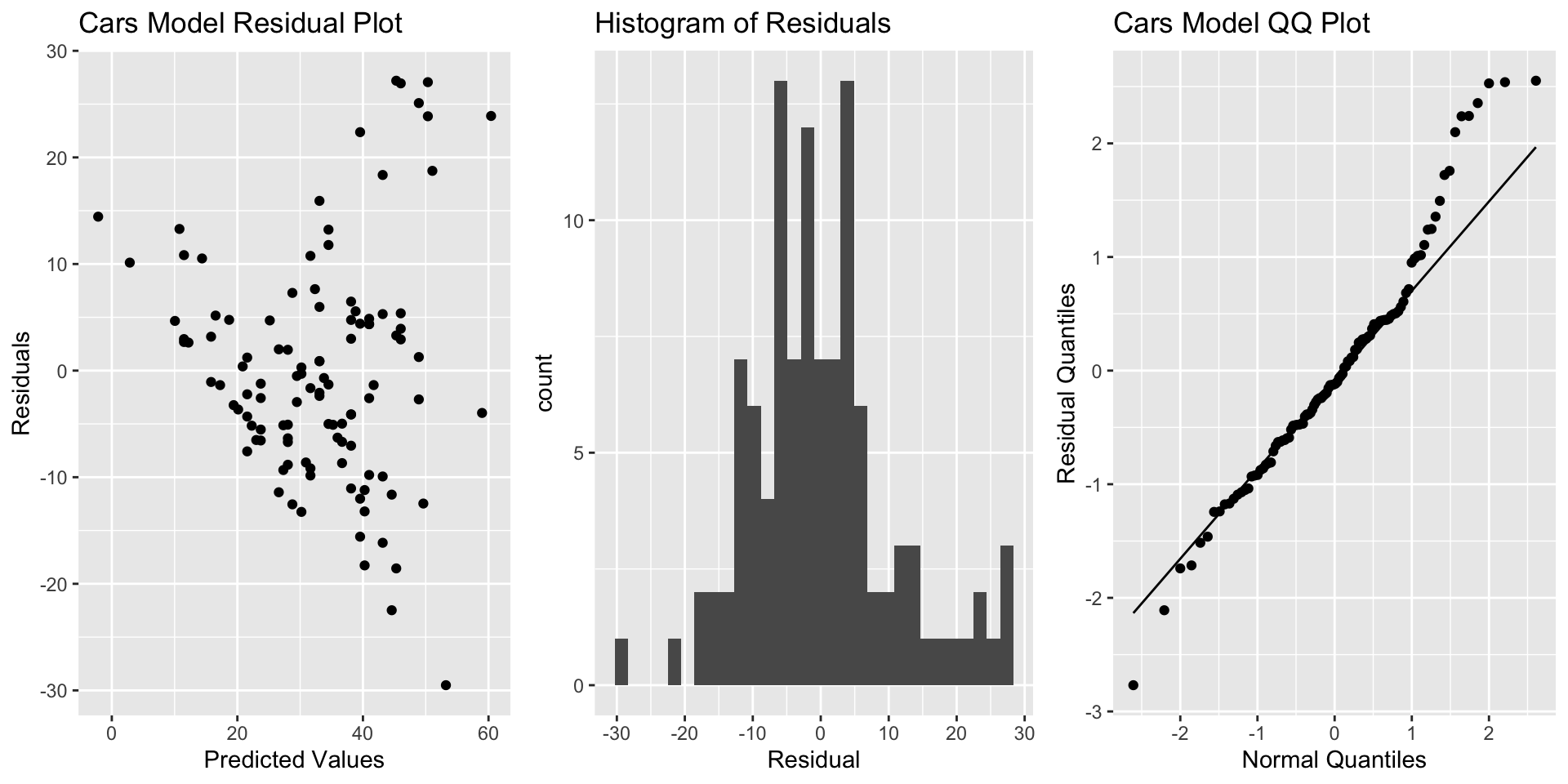
5.4 Section 5.4: Transformations
When residual plots reveal issues with model assumptions, we can try modeling a transformation of the response variable, such as log().
5.4.1 Model with Transformation
Cars_M_Log <- lm(data=Cars2015, log(LowPrice)~Acc060)
summary(Cars_M_Log)
##
## Call:
## lm(formula = log(LowPrice) ~ Acc060, data = Cars2015)
##
## Residuals:
## Min 1Q Median 3Q Max
## -0.84587 -0.19396 0.00908 0.18615 0.53350
##
## Coefficients:
## Estimate Std. Error t value Pr(>|t|)
## (Intercept) 5.13682 0.13021 39.45 <2e-16 ***
## Acc060 -0.22064 0.01607 -13.73 <2e-16 ***
## ---
## Signif. codes: 0 '***' 0.001 '**' 0.01 '*' 0.05 '.' 0.1 ' ' 1
##
## Residual standard error: 0.276 on 108 degrees of freedom
## Multiple R-squared: 0.6359, Adjusted R-squared: 0.6325
## F-statistic: 188.6 on 1 and 108 DF, p-value: < 2.2e-16When making predictions, we need to exponentiate.
exp(predict(Cars_M_Log, newdata=data.frame(Acc060=c(7)), interval="prediction", level=0.95))## fit lwr upr
## 1 36.31908 20.94796 62.96917Likewise, we are interested in \(e^{b_j}\).
exp(confint(Cars_M_Log))## 2.5 % 97.5 %
## (Intercept) 131.4610408 220.284693
## Acc060 0.7768669 0.827959