Chapter 4 Simulation-Based Hypothesis Tests
In a simulation-based hypothesis test, we test the null hypothesis of no relationship between one or more explanatory variables and a response variable.
4.1 Performing the Simulation-Based Test for Regression Coefficient
To test for a relationship between a response variable and a single quantitative explanatory variable, or a categorical variable with only two categories, we perform the following steps.
- Fit the model to the actual data and record the value of the regression coefficient \(b_1\), which describes the slope of the regression line (for a quantitative variable), or the difference between groups (for a categorical variable with 2 categories).
Repeat the following steps many (say 10,000) times, using a "for" loop:
Randomly shuffle the values (or categories) of the explanatory variable to create a scenario where there is no systematic relationship between the explanatory and response variable.
Fit the model to the shuffled data, and record the value of \(b_1\).
Observe how many of our simulations resulted in values of \(b_1\) as extreme as the one from the actual data. If this proportion is small, we have evidence that our result did not occur just by chance. If this value is large, it is plausible that the result we saw occurred by chance alone, and thus there is not enough evidence to say there is a relationship between the explanatory and response variables.
These steps are performed in the code below, using the example of price and acceleration time of 2015 cars.
4.1.1 Simulation-Based Hypothesis Test Example
Cars_M_A060  <- lm(data=Cars2015, LowPrice~Acc060)
b1 <- Cars_M_A060$coef[2] # record value of b1 from actual data
# perform simulation
b1Sim <- rep(NA, 10000)          # vector to hold results
ShuffledCars <- Cars2015    # create copy of dataset
for (i in 1:10000){
  #randomly shuffle acceleration times
ShuffledCars$Acc060 <- ShuffledCars$Acc060[sample(1:nrow(ShuffledCars))]
ShuffledCars_M<- lm(data=ShuffledCars, LowPrice ~ Acc060)   #fit model to shuffled data
b1Sim[i] <- ShuffledCars_M$coef[2]  # record b1 from shuffled model
}
Cars_A060SimulationResults <- data.frame(b1Sim)  #save results in dataframe
Now that we've performed the simulation, we'll display a histogram of the sampling distribution for \(b_1\) when the null hypothesis of no relationship between price and acceleration time is true.
b1 <- Cars_M_A060$coef[2] # record value of b1 from actual data
Cars_A060SimulationResultsPlot <- ggplot(data=Cars_A060SimulationResults, aes(x=b1Sim)) +
  geom_histogram(fill="lightblue", color="white") +
  geom_vline(xintercept=c(b1, -1*b1), color="red") +
  xlab("Simulated Value of b1") + ylab("Frequency") +
  ggtitle("Distribution of b1 under assumption of no relationship")
Cars_A060SimulationResultsPlot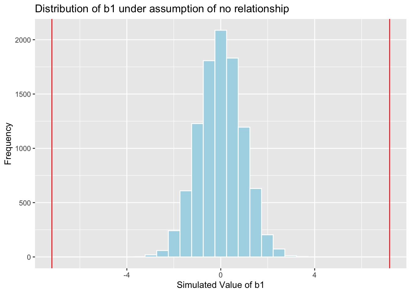
We can calculate the p-value by finding the proportion of simulations with \(b_1\) values more extreme than the observed value of \(b_1\), in absolute value.
mean(abs(b1Sim) > abs(b1))## [1] 04.2 Simulation-Based F-Test
When testing for a relationship between the response variable and a categorical variable with more than 2 categories, we first use the F-statistic to capture the maginitude of differences between groups. The process is similar to the one above, with the exception that we recored the value of F, rather than \(b_1\).
4.2.1 Simulation-Based F-Test Example
Cars_M_Size <- lm(data=Cars2015, LowPrice~Size)
Fstat <- summary(Cars_M_Size)$fstatistic[1] # record value of F-statistic from actual data
# perform simulation
FSim <- rep(NA, 10000)          # vector to hold results
ShuffledCars <- Cars2015    # create copy of dataset
for (i in 1:10000){
  #randomly shuffle acceleration times
ShuffledCars$Size <- ShuffledCars$Size[sample(1:nrow(ShuffledCars))]
ShuffledCars_M<- lm(data=ShuffledCars, LowPrice ~ Size)   #fit model to shuffled data
FSim[i] <- summary(ShuffledCars_M)$fstatistic[1]  # record F from shuffled model
}
CarSize_SimulationResults <- data.frame(FSim)  #save results in dataframe
Create the histogram of the sampling distribution for \(F\).
CarSize_SimulationResults_Plot <- ggplot(data=CarSize_SimulationResults, aes(x=FSim)) +
  geom_histogram(fill="lightblue", color="white") +
  geom_vline(xintercept=c(Fstat), color="red") +
  xlab("Simulated Value of F") + ylab("Frequency") +
  ggtitle("Distribution of F under assumption of no relationship")
CarSize_SimulationResults_Plot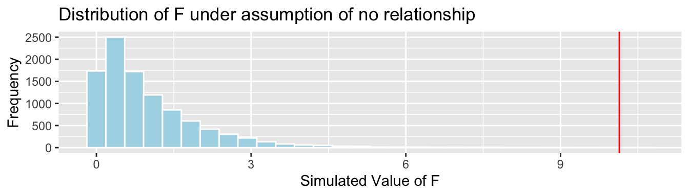
Calculate the p-value:
mean(FSim > Fstat)## [1] 1e-044.3 Testing for Differences Between Groups
If we find differences in the F-statistic, we should test for differences between individual groups, or categories.
In this example, those are given by \(b_1\), \(b_2\), and \(b_1-b_2\). When considering p-values, keep in mind that we are perfoming multiple tests simultaneously, so we should use a multiple-testing procedure, such as the Bonferroni correction.
4.3.1 Differences Between Groups Example
b1 <- Cars_M_Size$coefficients[2]  #record b1 from actual data
b2 <- Cars_M_Size$coefficients[3]  #record b2 from actual data
# perform simulation
b1Sim <- rep(NA, 10000)          # vector to hold results
b2Sim <- rep(NA, 10000)          # vector to hold results
ShuffledCars <- Cars2015    # create copy of dataset
for (i in 1:10000){
  #randomly shuffle acceleration times
ShuffledCars$Size <- ShuffledCars$Size[sample(1:nrow(ShuffledCars))]
ShuffledCars_M<- lm(data=ShuffledCars, LowPrice ~ Size)   #fit model to shuffled data
b1Sim[i] <- ShuffledCars_M$coefficients[2]   # record b1 from shuffled model
b2Sim[i] <- ShuffledCars_M$coefficients[3]   # record b2 from shuffled model
}
Cars_Size2_SimulationResults <- data.frame(b1Sim, b2Sim)  #save results in dataframe
Sampling Distribution for \(b_1\)
Cars_Size2_SimulationResultsPlot_b1 <- ggplot(data=Cars_Size2_SimulationResults, aes(x=b1Sim)) +
  geom_histogram(fill="lightblue", color="white") +
  geom_vline(xintercept=c(b1, -1*b1), color="red") +
  xlab("Simulated Value of b1") + ylab("Frequency") +
  ggtitle("Large vs Midsize Cars: Distribution of b1 under assumption of no relationship")
Cars_Size2_SimulationResultsPlot_b1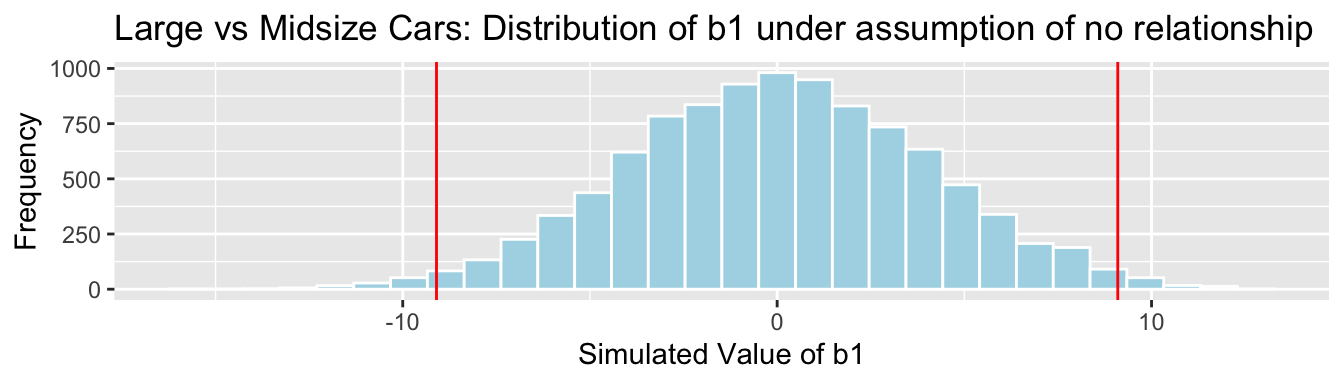
p-value:
mean(abs(b1Sim)>abs(b1))## [1] 0.0226Sampling Distribution for \(b_2\)
Cars_Size2_SimulationResultsPlot_b2 <- ggplot(data=Cars_Size2_SimulationResults, aes(x=b2Sim)) +
  geom_histogram(fill="lightblue", color="white") +
  geom_vline(xintercept=c(b2, -1*b2), color="red") +
  xlab("Simulated Value of b2") + ylab("Frequency") +
  ggtitle("Large vs Small Cars: Distribution of b2 under assumption of no relationship")
Cars_Size2_SimulationResultsPlot_b2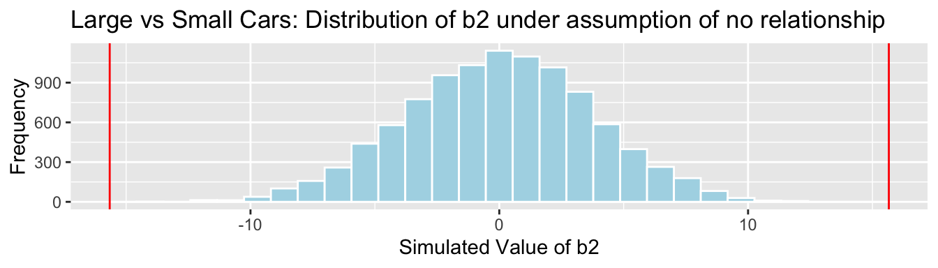
p-value:
mean(abs(b2Sim)>abs(b2))## [1] 0Sampling Distribution for \(b_1 - b_2\)
Cars_Size2_SimulationResultsPlot_b1_b2 <- ggplot(data=Cars_Size2_SimulationResults,
                                                 aes(x=b1Sim-b2Sim)) +
  geom_histogram(fill="lightblue", color="white") +
  geom_vline(xintercept=c(b1-b2, -1*(b1-b2)), color="red") +
  xlab("Simulated Value of b1-b2") + ylab("Frequency") +
  ggtitle("Small vs Midsize Cars: Distribution of b1-b2 under assumption of no relationship")
Cars_Size2_SimulationResultsPlot_b1_b2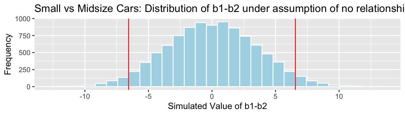
p-value:
mean(abs(b1Sim-b2Sim)>abs(b1-b2))## [1] 0.06294.4 "Theory-Based" Tests and Intervals in R
The quantity Pr(>|t|) in the coefficients table contains p-values pertaining to the test of the null hypothesis that that parameter is 0.
The confint() command returns confidence intervals for the regression model parameters.
The aov() command displays the F-statistic and p-value, as well as the sum of squared residuals and sum of squares explained by the model.
4.4.1 Example "Theory-Based" Test and Interval
summary(Cars_M_A060)##
## Call:
## lm(formula = LowPrice ~ Acc060, data = Cars2015)
##
## Residuals:
## Min 1Q Median 3Q Max
## -29.512 -6.544 -1.265 4.759 27.195
##
## Coefficients:
## Estimate Std. Error t value Pr(>|t|)
## (Intercept) 89.9036 5.0523 17.79 <2e-16 ***
## Acc060 -7.1933 0.6234 -11.54 <2e-16 ***
## ---
## Signif. codes: 0 '***' 0.001 '**' 0.01 '*' 0.05 '.' 0.1 ' ' 1
##
## Residual standard error: 10.71 on 108 degrees of freedom
## Multiple R-squared: 0.5521, Adjusted R-squared: 0.548
## F-statistic: 133.1 on 1 and 108 DF, p-value: < 2.2e-16confint(Cars_M_A060, level=0.95)## 2.5 % 97.5 %
## (Intercept) 79.888995 99.918163
## Acc060 -8.429027 -5.9576514.4.2 Example Theory-Based F-Test
summary(Cars_M_A060)##
## Call:
## lm(formula = LowPrice ~ Acc060, data = Cars2015)
##
## Residuals:
## Min 1Q Median 3Q Max
## -29.512 -6.544 -1.265 4.759 27.195
##
## Coefficients:
## Estimate Std. Error t value Pr(>|t|)
## (Intercept) 89.9036 5.0523 17.79 <2e-16 ***
## Acc060 -7.1933 0.6234 -11.54 <2e-16 ***
## ---
## Signif. codes: 0 '***' 0.001 '**' 0.01 '*' 0.05 '.' 0.1 ' ' 1
##
## Residual standard error: 10.71 on 108 degrees of freedom
## Multiple R-squared: 0.5521, Adjusted R-squared: 0.548
## F-statistic: 133.1 on 1 and 108 DF, p-value: < 2.2e-16Cars_A_Size <- aov(data=Cars2015, LowPrice~Size)
summary(Cars_A_Size)## Df Sum Sq Mean Sq F value Pr(>F)
## Size 2 4405 2202.7 10.14 9.27e-05 ***
## Residuals 107 23242 217.2
## ---
## Signif. codes: 0 '***' 0.001 '**' 0.01 '*' 0.05 '.' 0.1 ' ' 1confint(Cars_A_Size)## 2.5 % 97.5 %
## (Intercept) 36.88540 47.736327
## SizeMidsized -16.48366 -1.713069
## SizeSmall -22.55789 -8.759618