Chapter 6 Logistic Regression

We'll load the Default dataset used in the notes.

library(ISLR)
data(Default)
#convert default from yes/no to 0/1
Default$default <- as.numeric(Default$default=="Yes") 

6.1 Section 6.1: Visualizing the Logistic Curve

Template:

ggplot(data=Dataset_Name, aes(y=Response_Variable, x= Explanatory_Variable)) +
  geom_point(alpha=0.2) + 
  stat_smooth(method="glm", se=FALSE, method.args = list(family=binomial)) 

6.1.1 Visualizing Logistic Regression

ggplot(data=Default, aes(y=default, x= balance)) + geom_point(alpha=0.2) + 
  stat_smooth(method="glm", se=FALSE, method.args = list(family=binomial))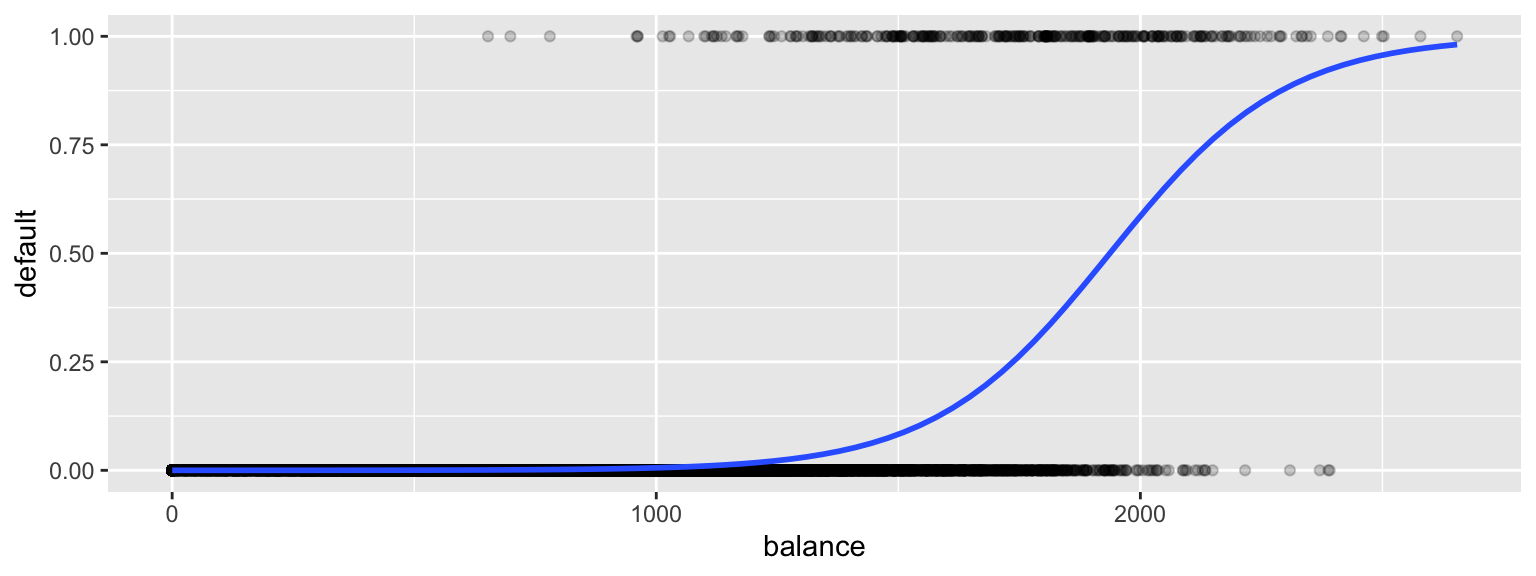 

6.2 Fitting Logistic Regression Model

6.2.1 Logistic Regression Template

Template:

M <- glm(data=Dataset_Name, Response_Variable ~ Explanatory_Variable, 
         family = binomial(link = "logit"))
summary(M)

6.2.2 Logistic Regression Example

CCDefault_M <- glm(data=Default, default ~ balance, family = binomial(link = "logit"))
summary(M)

## 
## Call:
## lm(formula = Weight ~ Age * Sex, data = Bears_Subset)
## 
## Residuals:
##      Min       1Q   Median       3Q      Max 
## -207.583  -38.854   -9.574   23.905  174.802 
## 
## Coefficients:
##             Estimate Std. Error t value Pr(>|t|)    
## (Intercept)  70.4322    17.7260   3.973 0.000219 ***
## Age           3.2381     0.3435   9.428 7.65e-13 ***
## Sex2        -31.9574    35.0314  -0.912 0.365848    
## Age:Sex2     -1.0350     0.6237  -1.659 0.103037    
## ---
## Signif. codes:  0 '***' 0.001 '**' 0.01 '*' 0.05 '.' 0.1 ' ' 1
## 
## Residual standard error: 70.18 on 52 degrees of freedom
##   (41 observations deleted due to missingness)
## Multiple R-squared:  0.6846, Adjusted R-squared:  0.6664 
## F-statistic: 37.62 on 3 and 52 DF,  p-value: 4.552e-13

6.2.3 Intervals and Predictions in Logistic Regression

The confint() command returns the model coefficient.

confint(CCDefault_M, level = 0.95)

##                     2.5 %       97.5 %
## (Intercept) -11.383288936 -9.966565064
## balance       0.005078926  0.005943365

Often, we are interested in \(e^{b_j}\). We can calculate this using exp()

exp(confint(CCDefault_M, level = 0.95))

##                    2.5 %       97.5 %
## (Intercept) 1.138415e-05 4.694353e-05
## balance     1.005092e+00 1.005961e+00

To obtain predictions as probabilities, use type="response".

predict(CCDefault_M, newdata=data.frame((balance=1000)), type="response")

##           1 
## 0.005752145