Chapter 7 Building Models for Interpretation
7.1 Plots for Model Selection
7.1.1 Correlation Matrix and Plot
Cars_Cat <- select_if(Cars2015, is.factor)
summary(Cars_Cat)
## Make Model Type Drive Size
## Chevrolet: 8 CTS : 2 7Pass :15 AWD:25 Large :29
## Ford : 7 2 Touring : 1 Hatchback:11 FWD:63 Midsized:34
## Hyundai : 7 200 : 1 Sedan :46 RWD:22 Small :47
## Toyoto : 7 3 i Touring: 1 Sporty :11
## Audi : 6 3 Series GT: 1 SUV :18
## Nissan : 6 300 : 1 Wagon : 9
## (Other) :69 (Other) :103Cars_Num <- select_if(Cars2015, is.numeric)
C <- cor(Cars_Num, use = "pairwise.complete.obs")
round(C,2)## LowPrice HighPrice CityMPG HwyMPG FuelCap Length Width Wheelbase
## LowPrice 1.00 0.91 -0.65 -0.59 0.57 0.47 0.48 0.46
## HighPrice 0.91 1.00 -0.56 -0.49 0.47 0.39 0.37 0.39
## CityMPG -0.65 -0.56 1.00 0.93 -0.77 -0.72 -0.78 -0.69
## HwyMPG -0.59 -0.49 0.93 1.00 -0.75 -0.64 -0.75 -0.64
## FuelCap 0.57 0.47 -0.77 -0.75 1.00 0.82 0.85 0.79
## Length 0.47 0.39 -0.72 -0.64 0.82 1.00 0.81 0.92
## Width 0.48 0.37 -0.78 -0.75 0.85 0.81 1.00 0.76
## Wheelbase 0.46 0.39 -0.69 -0.64 0.79 0.92 0.76 1.00
## Height 0.02 -0.10 -0.39 -0.54 0.58 0.46 0.62 0.49
## UTurn 0.40 0.31 -0.73 -0.68 0.76 0.84 0.77 0.81
## Weight 0.55 0.43 -0.83 -0.84 0.91 0.82 0.91 0.81
## Acc030 -0.76 -0.74 0.64 0.51 -0.47 -0.38 -0.41 -0.31
## Acc060 -0.74 -0.72 0.68 0.52 -0.49 -0.47 -0.46 -0.38
## QtrMile -0.76 -0.76 0.65 0.49 -0.45 -0.42 -0.41 -0.35
## PageNum -0.23 -0.20 0.28 0.15 -0.15 -0.23 -0.20 -0.24
## Height UTurn Weight Acc030 Acc060 QtrMile PageNum
## LowPrice 0.02 0.40 0.55 -0.76 -0.74 -0.76 -0.23
## HighPrice -0.10 0.31 0.43 -0.74 -0.72 -0.76 -0.20
## CityMPG -0.39 -0.73 -0.83 0.64 0.68 0.65 0.28
## HwyMPG -0.54 -0.68 -0.84 0.51 0.52 0.49 0.15
## FuelCap 0.58 0.76 0.91 -0.47 -0.49 -0.45 -0.15
## Length 0.46 0.84 0.82 -0.38 -0.47 -0.42 -0.23
## Width 0.62 0.77 0.91 -0.41 -0.46 -0.41 -0.20
## Wheelbase 0.49 0.81 0.81 -0.31 -0.38 -0.35 -0.24
## Height 1.00 0.55 0.71 0.21 0.21 0.25 0.06
## UTurn 0.55 1.00 0.80 -0.36 -0.41 -0.37 -0.22
## Weight 0.71 0.80 1.00 -0.41 -0.43 -0.39 -0.20
## Acc030 0.21 -0.36 -0.41 1.00 0.95 0.95 0.25
## Acc060 0.21 -0.41 -0.43 0.95 1.00 0.99 0.26
## QtrMile 0.25 -0.37 -0.39 0.95 0.99 1.00 0.26
## PageNum 0.06 -0.22 -0.20 0.25 0.26 0.26 1.00library(corrplot)
C <- corrplot(C)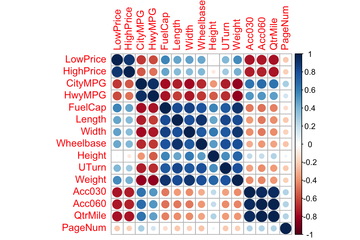
7.2 Residual by Explanatory Variable Plots
First, we fit a model:
Cars_M6 <- lm(data=Cars2015, log(LowPrice) ~ QtrMile + Weight + HwyMPG)
summary(Cars_M6)
##
## Call:
## lm(formula = log(LowPrice) ~ QtrMile + Weight + HwyMPG, data = Cars2015)
##
## Residuals:
## Min 1Q Median 3Q Max
## -0.82308 -0.14513 -0.01922 0.16732 0.41390
##
## Coefficients:
## Estimate Std. Error t value Pr(>|t|)
## (Intercept) 6.550e+00 4.220e-01 15.522 < 2e-16 ***
## QtrMile -2.170e-01 1.844e-02 -11.770 < 2e-16 ***
## Weight 1.592e-04 4.456e-05 3.573 0.000532 ***
## HwyMPG -9.611e-03 7.377e-03 -1.303 0.195410
## ---
## Signif. codes: 0 '***' 0.001 '**' 0.01 '*' 0.05 '.' 0.1 ' ' 1
##
## Residual standard error: 0.2198 on 106 degrees of freedom
## Multiple R-squared: 0.7732, Adjusted R-squared: 0.7668
## F-statistic: 120.5 on 3 and 106 DF, p-value: < 2.2e-167.2.1 Creating Residual by Explanatory Variable Plot
The code for residual by explanatory plot is shown. More plots can be added if there are additional explanatory variables.
P1 <- ggplot(data=data.frame(Cars_M6$residuals),
             aes(y=Cars_M6$residuals, x=Cars_M6$model$QtrMile)) +
  geom_point() + ggtitle("Cars Model Residual Plot") +
  xlab("Quarter Mile Time") + ylab("Residuals")
P2 <- ggplot(data=data.frame(Cars_M6$residuals),
             aes(y=Cars_M6$residuals, x=Cars_M6$model$Weight)) +
  geom_point() + ggtitle("Cars Model Residual Plot") +
  xlab("Weight") + ylab("Residuals")
grid.arrange(P1, P2, ncol=2)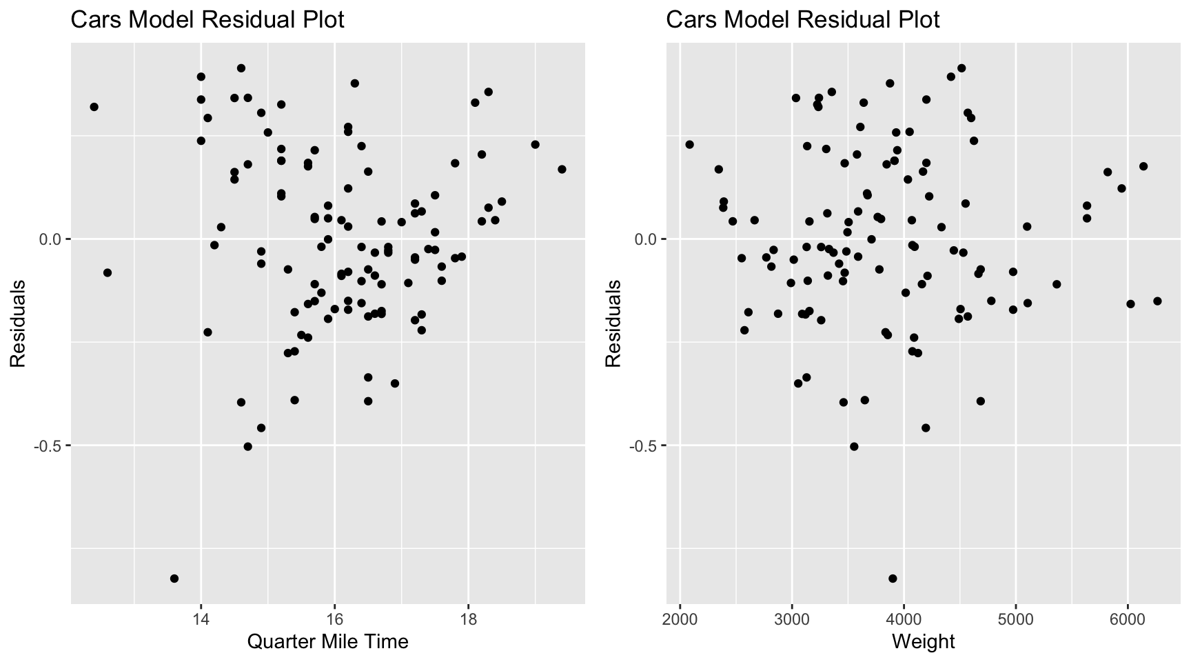
7.3 Section 7.3 Polynomial Regression
7.3.1 Plotting Polynomial Curves
ggplot(data=Cars2015, aes(y=LowPrice, x=FuelCap)) +
  geom_point()+ stat_smooth(method="lm", se=FALSE) +
  stat_smooth(method="lm", se=TRUE, fill=NA,formula=y ~ poly(x, 2, raw=TRUE),colour="red") +
  stat_smooth(method="lm", se=TRUE, fill=NA,formula=y ~ poly(x, 3, raw=TRUE),colour="green") +
  stat_smooth(method="lm", se=TRUE, fill=NA,formula=y ~ poly(x, 4, raw=TRUE),colour="orange") +
  stat_smooth(method="lm", se=TRUE, fill=NA,formula=y ~ poly(x, 5, raw=TRUE),colour="purple") +
  stat_smooth(method="lm", se=TRUE, fill=NA,formula=y ~ poly(x, 6, raw=TRUE),colour="darkgreen")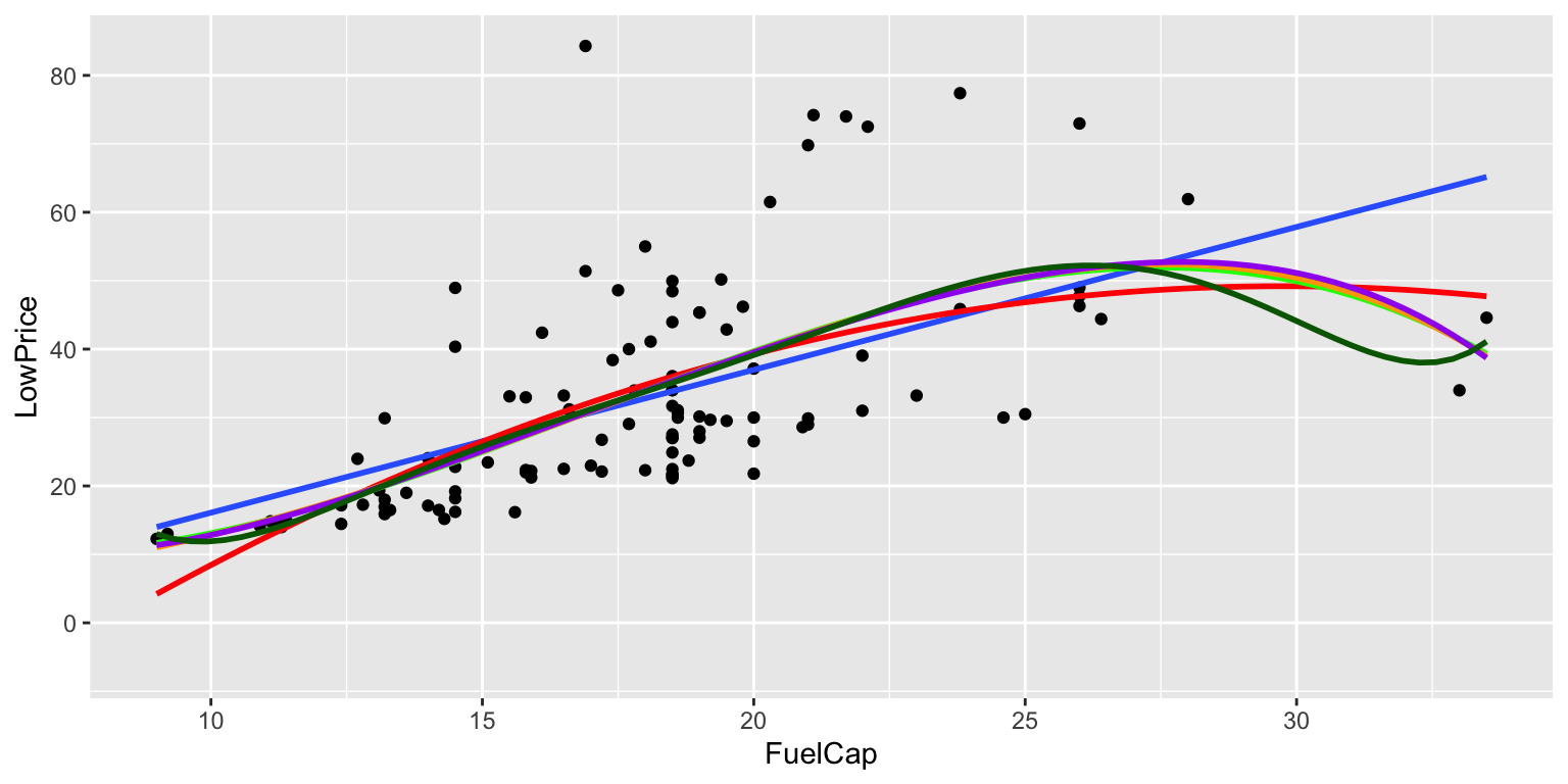
7.3.2 Fitting Polynomial Models
To fit a model with higher powers, use I(Variable^k).
CarLength_M1 <- lm(data=Cars2015, LowPrice~FuelCap)
CarLength_M2 <- lm(data=Cars2015, LowPrice~FuelCap + I(FuelCap^2))
CarLength_M3 <- lm(data=Cars2015, LowPrice~FuelCap + I(FuelCap^2) + I(FuelCap^3))
CarLength_M4 <- lm(data=Cars2015, LowPrice~FuelCap + I(FuelCap^2) + I(FuelCap^3) + I(FuelCap^4))
CarLength_M5 <- lm(data=Cars2015, LowPrice~FuelCap + I(FuelCap^2) + I(FuelCap^3) + I(FuelCap^4) +
                     I(FuelCap^5))
CarLength_M6 <- lm(data=Cars2015, LowPrice~FuelCap + I(FuelCap^2) + I(FuelCap^3) + I(FuelCap^4) +
                     I(FuelCap^5)+ I(FuelCap^6))
We can view the model summary, using the summary() command, as usual.
7.4 Adjusted \(R^2\), AIC, and BIC
We'll calculate ddjusted \(R^2\), AIC, and BIC, for Model M6, above.
7.4.1 Example: Calculating adjusted \(R^2\), AIC, and BIC
summary(CarLength_M6)$adj.r.squared## [1] 0.3573088AIC(CarLength_M6)## [1] 881.2588BIC(CarLength_M6)## [1] 902.8627