Chapter 3 Interval Estimation via Simulation
3.1 Performing the Bootstrap
Bootstrapping is a computationally-intense, simulation approach, designed to quantify variability associated with a statistic when generalizing from a sample to a large population.
To write code for a bootstrap, follow these steps
- Create vectors in which to store the bootstrap results. Create a vector for each statistic of interest.
- Write a for-loop in which you will perform a procedure many times (10000 simulations is usually appropriate in this class) within the loop perform steps 3 and 4.
- Take a sample the same size as the original data, using replacement.
- Calculate whatever statistics you are interested in for the bootstrap sample. This might involve calculating means, medians, standard deviations, or other statistics, or fitting a model to obtain regression coefficients.
- Combine results for each of the qualities you bootstrapped into a dataframe.
3.1.1 Setting a Seed
Because bootstrapping involves taking a random sample, results will come out slightly differentely each time you run your code. Doing a large number of simulations ensures that the average results from each simulation will be similar, but they will not be identical.
Thus, each time you knit your document, you'll get slightly different results, which can be a problem when summarizing your results. To avoid this, you can set a random seed, which tells R to start its random procedure in the same place each time. This is done using the set.seed() function. I typically use the date as my seed, but you can use any number you want.
set.seed(09262020)3.1.2 Template for Bootstrap
statistic1 <- rep(NA, 10000) # create vector to store bootstrap results for first statistic
statistic2 <- rep(NA, 10000) # create vector to store bootstrap results for second statistic
statistic3 <- rep(NA, 10000) # create vector to store bootstrap results for third statistic
# continue if there are more than 3 quantities of interest

# for loop
for (i in 1:10000){
BootstrapSample <- sample_n(DatasetName, samplesize, replace=TRUE)
statistic1[i] <- #calculate first statistic on bootstrap sample
statistic2[i] <- #calculate second statistic on bootstrap sample
statistic3[i] <- #calculate third statistic on bootstrap sample
}

Bootstrap_Results <- data.frame(statistic1, statistic2, statistic3)
3.1.3 Bootstrap for Proportion of Blue M&M's
Color <- c(rep("Blue", 6), rep("Orange", 3), rep("Green", 2), rep("Yellow", 2),
           rep("Red", 1))
Sample <- data.frame(Color)

Proportion_Blue <- rep(NA, 10000)
for (i in 1:10000){
BootstrapSample <- sample_n(Sample, 14, replace=TRUE)
Proportion_Blue[i] <- sum(BootstrapSample$Color=="Blue")/14
}
Candy_Bootstrap_Results <- data.frame(Proportion_Blue)
3.1.4 Bootstrap for Mean, Median, St.Dev., Prop>1
Bootstrap mean, median, standard deviation, mercury levels in Florida lakes, and percentage of lakes with mercury level exceeding 1 ppm.
MeanHg <- rep(NA, 10000)
StDevHg <- rep(NA, 10000)
PropOver1 <- rep(NA, 10000)
MedianHg <- rep(NA, 10000)

for (i in 1:10000){
BootstrapSample <- sample_n(FloridaLakes, 53, replace=TRUE)
MeanHg[i] <- mean(BootstrapSample$AvgMercury)
StDevHg[i] <- sd(BootstrapSample$AvgMercury)
PropOver1[i] <- mean(BootstrapSample$AvgMercury>1)
MedianHg[i] <- median(BootstrapSample$AvgMercury)
}
Lakes_Bootstrap_Results <- data.frame(MeanHg, MedianHg, PropOver1, StDevHg)
3.1.5 Bootstrap for Difference Between Groups
Consider the difference between average mercury levels in northern and southern Florida lakes. First, we'll add the location variable to the dataset.
library(Lock5Data)
data(FloridaLakes)
#Location relative to rt. 50
FloridaLakes$Location <- as.factor(c("S","S","N","S","S","N","N","N","N","N","N",
                                     "S","N","S","N","N","N","N","S","S","N","S",
                                     "N","S","N","S","N","S","N","N","N","N","N",
                                     "N","S","N","N","S","S","N","N","N","N","S",
                                     "N","S","S","S","S","N","N","N","N"))
head(FloridaLakes %>% select(Lake, AvgMercury, Location))
## # A tibble: 6 x 3
## Lake AvgMercury Location
## <chr> <dbl> <fct>
## 1 Alligator 1.23 S
## 2 Annie 1.33 S
## 3 Apopka 0.04 N
## 4 Blue Cypress 0.44 S
## 5 Brick 1.2 S
## 6 Bryant 0.27 NWhen performing the bootstrap, we sample the same number of observations from each category as were present in the original data. In this example, there were 33 lakes in Northern Florida, and 20 in Southern Florida. We'll fit a model with the categorical explanatory variable, location, and recall that \(b_1\) represents the average difference between northern and southern lakes. We'll bootstrap for the distribution of \(b_1\).
b1 <- rep(NA, 10000)  #vector to store b1 values
for (i in 1:10000){
NLakes <- sample_n(FloridaLakes %>% filter(Location=="N"), 33, replace=TRUE)   # sample 33 northern lakes
SLakes <- sample_n(FloridaLakes %>% filter(Location=="S"), 20, replace=TRUE)   # sample 20 southern lakes
BootstrapSample <- rbind(NLakes, SLakes)   # combine Northern and Southern Lakes
M <- lm(data=BootstrapSample, AvgMercury ~ Location) # fit linear model
b1[i] <- coef(M)[2] # record b1 (note indexing in coefficents starts at 1, so b0=coef(M)[1], and b1=coef(M)[2], etc.)
}
NS_Lakes_Bootstrap_Results <- data.frame(b1)  #save results as dataframe
3.1.6 Bootstrap for Regression Coefficients
We'll bootstrap for coefficients in the bears interaction model.
b0 <- rep(NA, 10000)
b1 <- rep(NA, 10000)
b2 <- rep(NA, 10000)
b3 <- rep(NA, 10000)
for (i in 1:10000){
BootstrapSample <- sample_n(Bears_Subset, 97, replace=TRUE) #take bootstrap sample
M <- lm(data=BootstrapSample, Weight ~ Age*Sex) # fit linear model
b0[i] <- coef(M)[1] # record b0 (note indexing in coefficents starts at 1, so b0=coef(M)[1], and b1=coef(M)[2], etc.)
b1[i] <- coef(M)[2] # record b1
b2[i] <- coef(M)[3] # record b2
b3[i] <- coef(M)[4] # record b3
}
Bears_Bootstrap_Results <- data.frame(b0, b1, b2, b3)
3.2 Bootstrap Confidence Intervals
3.2.1 Visualizing the Bootstrap Distribution
Template for creating a histogram of the bootstrap distribution:
Boot_Dist_Plot <- ggplot(data=Bootstrap_Results, aes(x=statistic)) +
  geom_histogram(color="colorchoice", fill="colorchoice") +
  xlab("Statistic") + ylab("Frequency") +
  ggtitle("Bootstrap Distribution for ...")
Boot_Dist_Plot
3.2.2 Percentile Confidence Intervals
The quantile commands can be used to find the middle 95% of the bootstrap distribution. (or whatever percentage is desired).
q.025 <- quantile(Bootstrap_Results$statistic, 0.025)
q.975 <- quantile(Bootstrap_Results$statistic, 0.975)
c(q.025, q.975)
We can add the cutoff points of the percentile confidence interval to the plot, as shown.
Boot_Dist_Plot + geom_vline(xintercept=c(Estimate - 2*SE, Estimate + 2*SE), color="red")3.2.3 Standard Error Confidence Intervals
When the bootstrap distribution is symmetric and bell-shaped, the 2-standard error method also provides a reasonable confidence interval.
Calculate standard error:
SE <- sd(Bootstrap_Results$statistic)Calculate estimate from original sample
Estimate <- #calculate statistic of interest from original datasetAdd and subtract 2 standard errors
c(Estimate - 2*SE, Estimate + 2*SE)We add the cutoff points for the standard error confidence interval
Boot_Dist_Plot + geom_vline(xintercept = c(Estimate - 2*SE, Estimate + 2*SE), color="red")3.2.4 M&M Proportions
Boot_Dist_Plot <- ggplot(data=Candy_Bootstrap_Results, aes(x=Proportion_Blue)) + geom_histogram(fill="blue", color="white")
Boot_Dist_Plot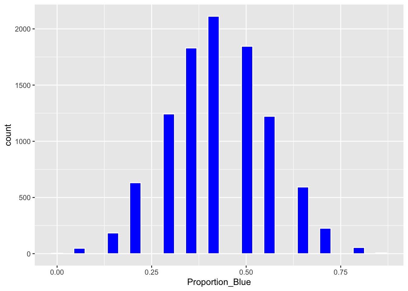
We calculate the 0.025 and 0.975 quantiles of the bootstrap distribution.
q.025 <- quantile(Candy_Bootstrap_Results$Proportion_Blue, 0.025)
q.975 <- quantile(Candy_Bootstrap_Results$Proportion_Blue, 0.975)
c(q.025, q.975)
## 2.5% 97.5%
## 0.2142857 0.7142857Plot of bootstrap distribution with percentile confidence interval endpoints.
Boot_Dist_Plot + geom_vline(xintercept=c(q.025, q.975), color="red")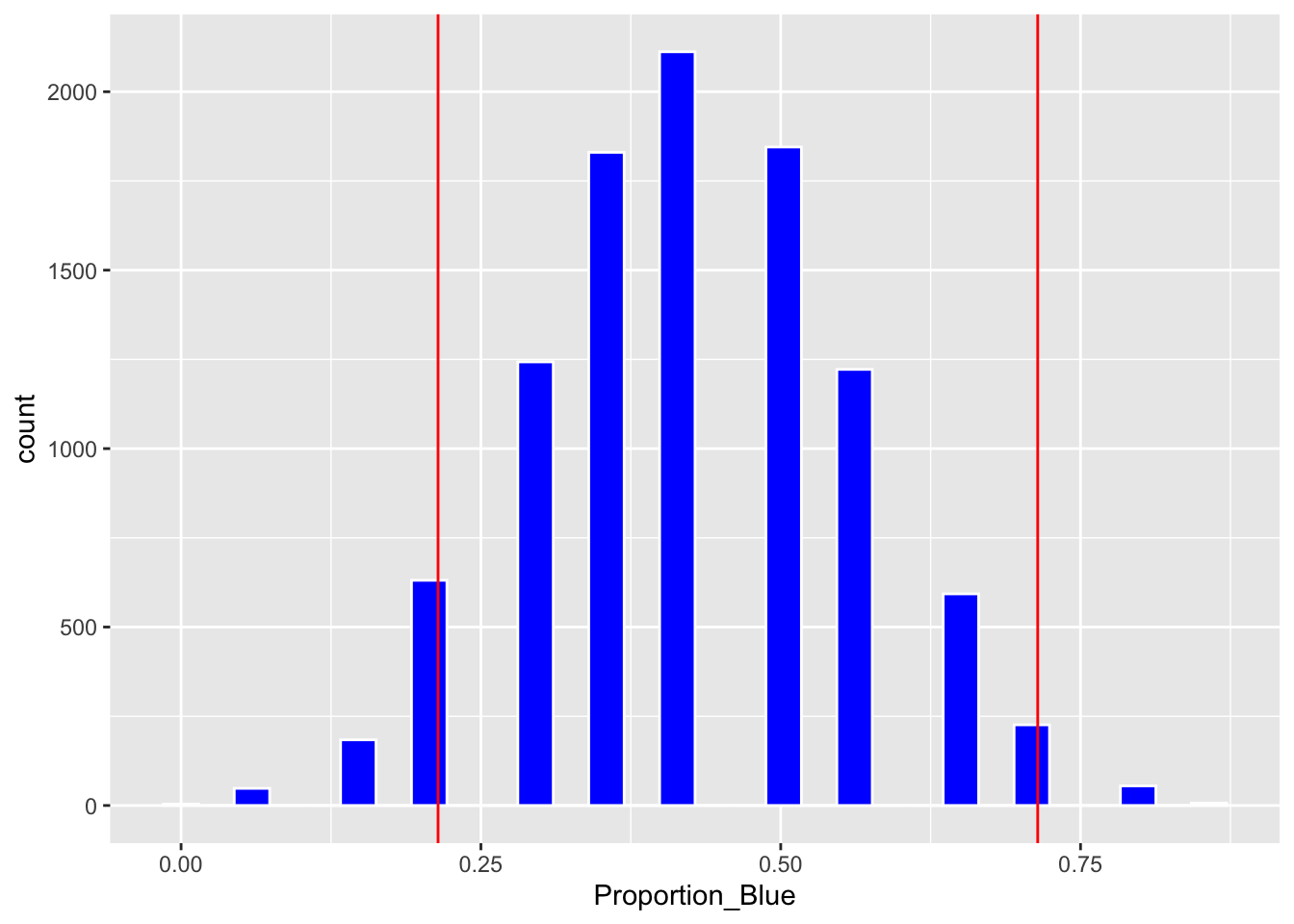
We'll calculate the standard deviation of the bootstrap distribution, also known as the bootstrap standard error.
SE <- sd(Candy_Bootstrap_Results$Proportion_Blue)
SE
## [1] 0.1318719A 95% standard error confidence interval is given by:
Estimate <- 6/14c(Estimate - 2*SE, Estimate + 2*SE)## [1] 0.1648277 0.6923152Boot_Dist_Plot + geom_vline(xintercept=c(Estimate - 2*SE, Estimate + 2*SE), color="red")
3.2.5 Bootstrap Distribution for Mean Mercury Level in Florida Lakes
Graph the bootstrap distribution:
Boot_Dist_Plot <- ggplot(data=Lakes_Bootstrap_Results, aes(x=MeanHg)) +
  geom_histogram(color="white", fill="blue") +
  xlab("Mean Mercury Level in Bootstrap Samples") + ylab("Frequency") +
  ggtitle("Bootstrap Distribution for Mean Mercury Level")
Boot_Dist_Plot
Calculate 0.025 and 0.975 quantiles:
q.025 <- quantile(Lakes_Bootstrap_Results$MeanHg, 0.025)
q.975 <- quantile(Lakes_Bootstrap_Results$MeanHg, 0.975)
c(q.025, q.975)
## 2.5% 97.5%
## 0.4394340 0.6215094Add cutoff points of interval to the plot:
Boot_Dist_Plot + geom_vline(xintercept=c(q.025, q.975), color="red")
Calculate standard error:
SE <- sd(Lakes_Bootstrap_Results$MeanHg)
SE
## [1] 0.04615476Calculate estimate from original sample
Estimate <- mean(FloridaLakes$AvgMercury)Add and subtract 2 standard errors
c(Estimate - 2*SE, Estimate + 2*SE)## [1] 0.4348603 0.6194793Plot with endpoints of SE Confidence interval
Boot_Dist_Plot + geom_vline(xintercept = c(Estimate - 2*SE, Estimate + 2*SE),
                            color="red")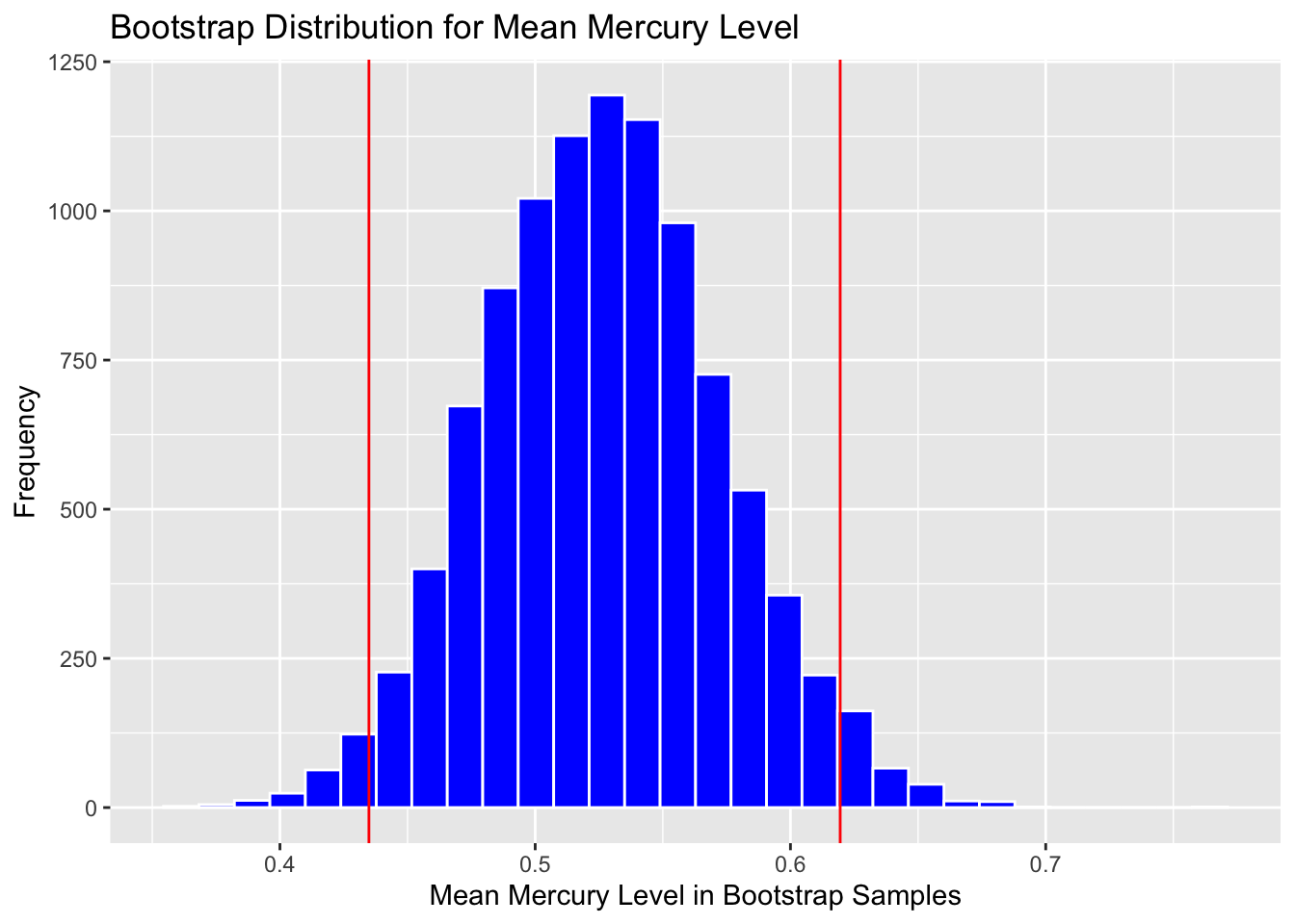
3.2.6 Bootstrap Distribution for Difference in Mean Mercury Level in Florida Lakes between N and S
Graph the bootstrap distribution:
Boot_Dist_Plot <- ggplot(data=NS_Lakes_Bootstrap_Results, aes(x=b1)) +
  geom_histogram(color="white", fill="blue") +
  xlab("Mean Difference in Mercury Level in Bootstrap Samples") + ylab("Frequency") +
  ggtitle("Bootstrap Distribution for Difference in  Mean Mercury Level for N vs S")
Boot_Dist_Plot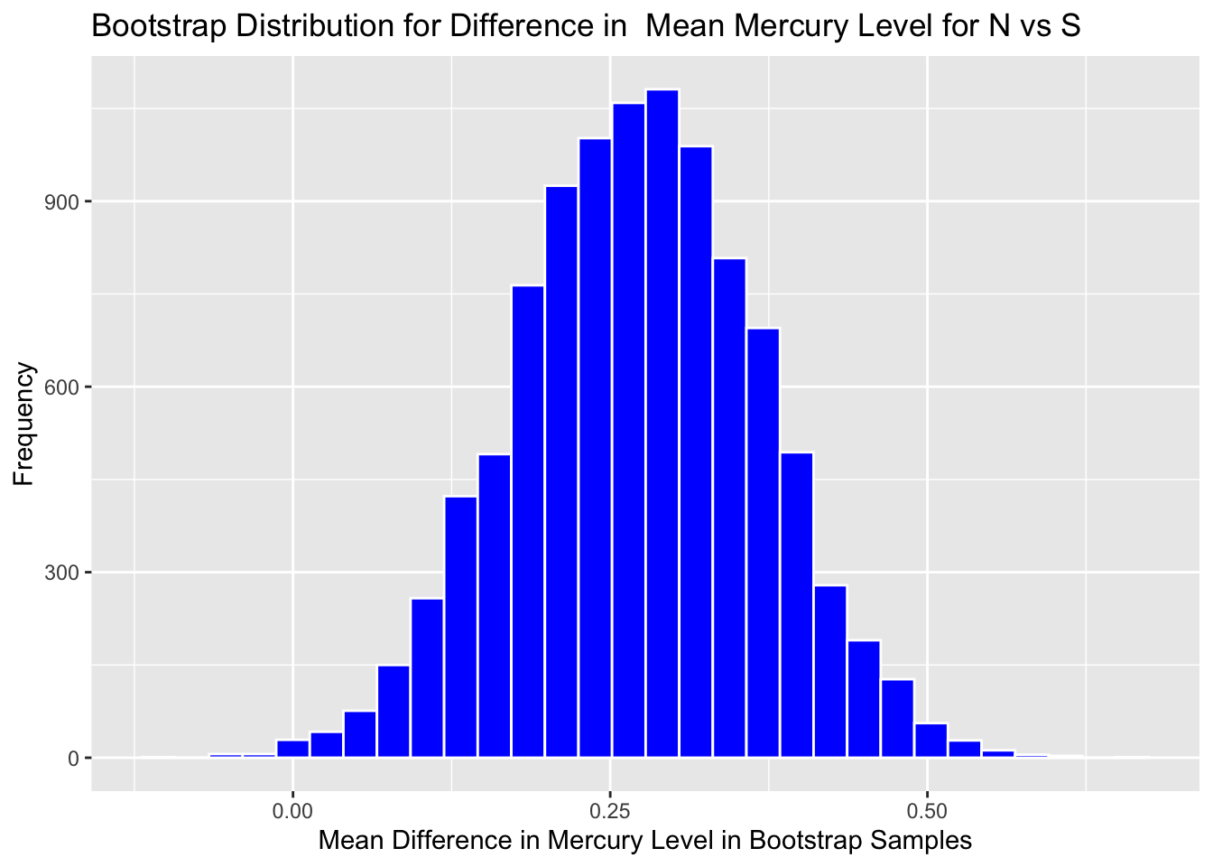
Calculate 0.025 and 0.975 quantiles:
q.025 <- quantile(NS_Lakes_Bootstrap_Results$b1, 0.025)
q.975 <- quantile(NS_Lakes_Bootstrap_Results$b1, 0.975)
c(q.025, q.975)
## 2.5% 97.5%
## 0.08442955 0.46011061Add cutoff points of interval to the plot:
Boot_Dist_Plot + geom_vline(xintercept=c(q.025, q.975), color="red")
Calculate standard error:
SE <- sd(NS_Lakes_Bootstrap_Results$b1)
SE
## [1] 0.09587673Calculate estimate from original sample:
M <- lm(data=FloridaLakes, AvgMercury~Location)
Estimate <- M$coef[2]  #record b1 from actual sample
Add and subtract 2 standard errors:
c(Estimate - 2*SE, Estimate + 2*SE)## LocationS LocationS
## 0.08020109 0.46370800Boot_Dist_Plot + geom_vline(xintercept=c(Estimate - 2*SE, Estimate + 2*SE), color="red")
3.2.7 Bootstrap Distribution for Coefficients in Bears Multiple Regression Model
We'll look at the bootstrap distribution for \((b_0 + b_2) + 24(b_1+b_3)\) which represents the expected weight of a 24 month old female bear.
Boot_Dist_Plot <- ggplot(data=Bears_Bootstrap_Results,
                         aes(x=b0+b2+24*(b1+b3))) +
  geom_histogram(color="white", fill="blue") +
  xlab("Mean Expected Weight in Bootstrap Samples") +
  ylab("Frequency") +
  ggtitle("Bootstrap Distribution for Expected Weight of 24 Month old Female Bear")
Boot_Dist_Plot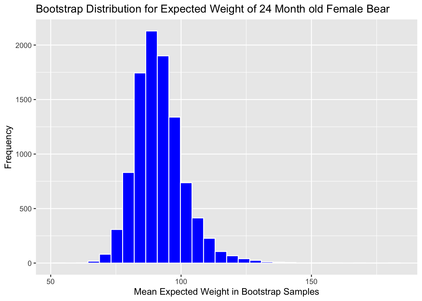
Calculate 0.025 and 0.975 quantiles:
q.025 <- quantile(Bears_Bootstrap_Results$b0 + Bears_Bootstrap_Results$b2 +
                    24*(Bears_Bootstrap_Results$b1 + Bears_Bootstrap_Results$b3), 0.025)
q.975 <- quantile(Bears_Bootstrap_Results$b0 + Bears_Bootstrap_Results$b2 +
                    24*(Bears_Bootstrap_Results$b1 + Bears_Bootstrap_Results$b3), 0.975)
c(q.025, q.975)
## 2.5% 97.5%
## 75.9636 113.5394Add cutoff points of interval to the plot:
Boot_Dist_Plot + geom_vline(xintercept=c(q.025, q.975), color="red")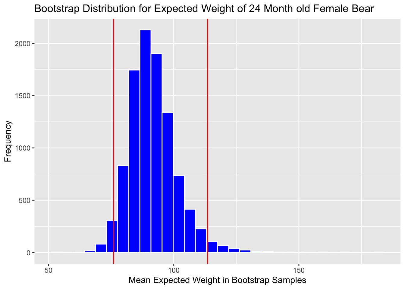
Calculate standard error:
SE <- sd(Bears_Bootstrap_Results$b0 + Bears_Bootstrap_Results$b2 +
                    24*(Bears_Bootstrap_Results$b1 + Bears_Bootstrap_Results$b3))
SE
## [1] 9.589441Calculate estimate from original sample:
M <- lm(data=Bears_Subset, Weight~Age*Sex)
Estimate <- M$coef[1] + M$coef[3] + 24*(M$coef[2]+M$coef[4])
Add and subtract 2 standard errors:
c(Estimate - 2*SE, Estimate + 2*SE)## (Intercept) (Intercept)
## 72.17105 110.52881Boot_Dist_Plot + geom_vline(xintercept=c(Estimate - 2*SE, Estimate + 2*SE),
color="red")
Note that the standard error method is not appropriate here, due to the right-skeweness in the bootstrap distribution.
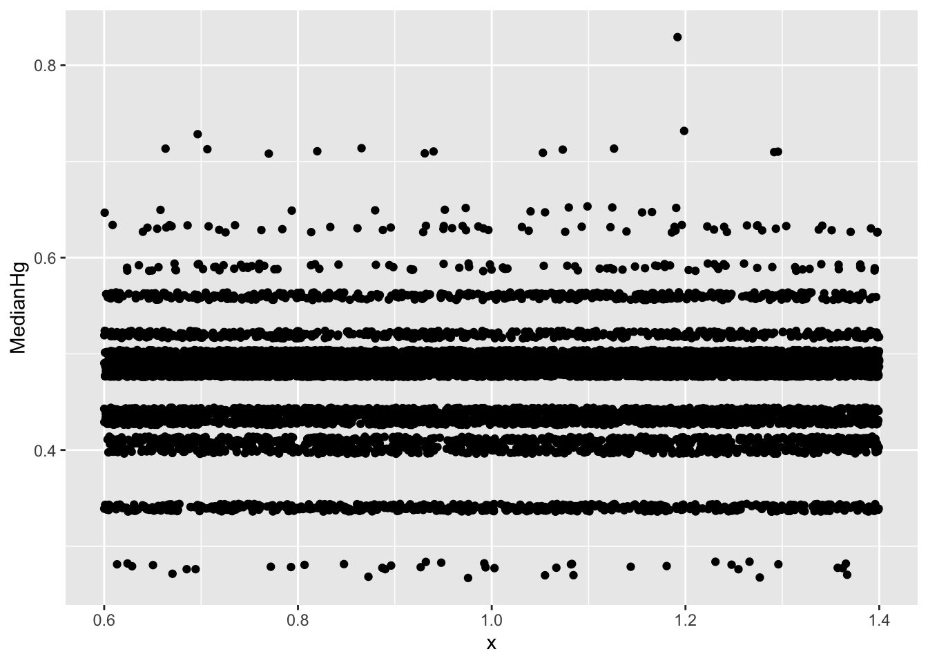
3.3 Checking for Gaps and Clusters
If there are gaps and/or clusters in the bootstrap distribution, it is inappropriate to create any kind of bootstrap confidence intervals. This is sometimes hard to tell from a histogram, as the choice of binwidth might lead to gaps that aren't really there in the bootstrap distribution. We can use jitter plots to look for gaps or clusters in the bootstrap distribution.
To do this, create a jitterplot, with the statistic from the bootstrap distribution on the y-axis. Simply say x=1, so there is an x-variable. The geom_jitter() command will spread the points out so they are not all on top of one another, and we can see them.
3.3.1 Example: When the Bootstrap is Inappropriate
ggplot(data=Lakes_Bootstrap_Results, aes(y=MedianHg, x=1)) + geom_jitter()