Chapter 1 Exploratory Data Analysis
This chapter describes how to load data into R, and explore its properties. The purpose of an exploratory data analysis (EDA) is to learn about the nature of the data, and to become aware of any surprising characteristics or anomalies that might impact our analysis and conclusions. An EDA typically involves calculating summary statistics, and creating graphs and tables that help us explore the data. It does not involve more advanced techniques, such as modeling, but rather helps set the stage for these to be done effectively.
As you explore the data, look for:
- Missing values
- Unusual observations
- Misspecified variable types
We'll begin by loading the tidyverse package, which can be used to create professional graphics, and wrangle (or manipulate) data into forms that are informative and easy to work with.
library(tidyverse)1.1 Section 1.1: Reading in Data
There are many ways to read data into R. We'll look at how to read data from common .csv, .txt, and .xlsx files, as well as how to load data that is already part of an R package. Knowing how to read data in these formats is sufficient for this class, however, there are other data formats that can be read into R. If you find yourself working with data in other forms, there are plenty of online resources available.
1.1.1 Read data from a local file on your computer.
If the data are in a .csv, .txt, .xlsx, or .xls file on your computer, make sure that the file is in the same directory as your .Rmd file, and that this is set as your working directory. The easiest way to accomplish this is by using an R Project. Then, read in the data, using read_csv() for .csv files, read_delim for .txt files, or read_excel for .xlsx or .xls files.
The filename goes in quotes inside the read function. The name on the left is the name you will give the dataset. You will use this to refer to the data in all future commands. The <- is called an assignment operator. It assigns the dataset you have read in to the name you are giving it.
1.1.2 Reading Data from a Directory on Your Computer
HollywoodMovies <- read.csv("HollywoodMovies.csv")HollywoodMovies <- read.delim("HollywoodMovies.txt")Reading in excel files requires loading the readxl package.
library(readxl)
HollywoodMovies <- read.excel("HollywoodMovies.xlsx")
1.1.3 Read data from the web
If reading data from the web, be sure to specify the entire url.
HollywoodMovies <- read.csv("https://www.lock5stat.com/datapage2e/HollywoodMovies.csv")HollywoodMovies <- read.csv("https://www.lock5stat.com/datapage2e/HollywoodMovies.txt")library(readxl)
HollywoodMovies <- read.csv("https://www.lock5stat.com/datapage2e/HollywoodMovies.xlsx")1.1.4 Load data already included in R package
If the dataset is already available in an R package, load that package and read in the data, using the data command.
library(Lock5Data)
data("HollywoodMovies")
1.1.5 R Help File
If your data are part of an R package, you can view the help file, containing information on the dataset using the command ? before the name of the dataset. This should open the description file in the lower right panel of the RStudio window. Even if your data are not part of an R package, it is a good idea to look for this kind of information if it is available.
?HollywoodMovies1.2 Preview the Data
The glimpse() function gives an overview of the information contained in a dataset. We can see the number of observations (rows), and the number of variables, (columns). We also see the name of each variable and its type. Variable types include
Categorical variables, which take on groups or categories, rather than numeric values. In R, these might be coded as logical
<logi>, character<chr>, factor<fct>and ordered factor<ord>.Quantitative variables, which take on meaningful numeric values. These include numeric
<num>, integer<int>, and double<dbl>.
1.2.1 glimpse()
glimpse(HollywoodMovies)## Rows: 1,295
## Columns: 15
## $ Movie <chr> "2016: Obama's America", "21 Jump Street", "A Late Qu…
## $ LeadStudio <chr> "Rocky Mountain Pictures ", "Sony Pictures Releasing …
## $ RottenTomatoes <int> 26, 85, 76, 90, 35, 27, 91, 56, 11, 44, 93, 63, 87, 9…
## $ AudienceScore <int> 73, 82, 71, 82, 51, 72, 62, 47, 47, 63, 82, 51, 63, 9…
## $ Genre <chr> "Documentary", "Comedy", "Drama", "Drama", "Horror", …
## $ TheatersOpenWeek <int> 1, 3121, 9, 7, 3108, 3039, 132, 245, 2539, 3192, 3, 1…
## $ OpeningWeekend <dbl> 0.03, 36.30, 0.08, 0.04, 16.31, 24.48, 1.14, 0.70, 11…
## $ BOAvgOpenWeekend <int> 30000, 11631, 8889, 5714, 5248, 8055, 8636, 2857, 449…
## $ Budget <dbl> 3.0, 42.0, NA, NA, 68.0, 12.0, NA, 7.5, 35.0, 50.0, 1…
## $ DomesticGross <dbl> 33.35, 138.45, 1.56, 1.55, 37.52, 70.01, 1.99, 3.01, …
## $ WorldGross <dbl> 33.35, 202.81, 6.30, 7.60, 137.49, 82.50, 3.59, 8.54,…
## $ ForeignGross <dbl> 0.00, 64.36, 4.74, 6.05, 99.97, 12.49, 1.60, 5.53, 9.…
## $ Profitability <dbl> 1334.00, 482.88, NA, NA, 202.19, 687.50, NA, 113.87, …
## $ OpenProfit <dbl> 1.20, 86.43, NA, NA, 23.99, 204.00, NA, 9.33, 32.57, …
## $ Year <int> 2012, 2012, 2012, 2012, 2012, 2012, 2012, 2012, 2012,…A function similar to glimpse() is skim(), which is part of the skimr() package. skim() shows us:
For factor variables, skimr() reports
* number of missing cases (emp)
* proportion of complete cases, i.e. not missing (complete_rate)
* whether or not the categories have an ordering (ordered)
* number of unique categories (n_unique)
* most frequently occurring (top_counts)
For numeric variables, skimr() reports
* number of missing values (n_missing)
* proportion of complete cases, i.e. not missing (complete_rate)
* mean
* standard deviation (sd)
* minimum (p0), 25th percentile (p25), median (p50), 75th percentile (p75), and maximum (p100)
* a histogram of the values (these can be hard to read)
1.2.1.1 summary()
The summary function provides additional information. It can be used for the entire dataset, or individual variables.
summary(HollywoodMovies)## Movie LeadStudio RottenTomatoes AudienceScore
## Length:1295 Length:1295 Min. : 0.00 Min. :10.00
## Class :character Class :character 1st Qu.:33.00 1st Qu.:49.00
## Mode :character Mode :character Median :61.00 Median :64.00
## Mean :57.58 Mean :62.18
## 3rd Qu.:84.00 3rd Qu.:77.00
## Max. :99.00 Max. :99.00
## NA's :6
## Genre TheatersOpenWeek OpeningWeekend BOAvgOpenWeekend
## Length:1295 Min. : 1.0 Min. : 0.020 Min. : 204
## Class :character 1st Qu.: 152.5 1st Qu.: 0.845 1st Qu.: 3482
## Mode :character Median :2459.0 Median : 7.600 Median : 6586
## Mean :2008.0 Mean : 17.541 Mean : 13400
## 3rd Qu.:3213.5 3rd Qu.: 20.810 3rd Qu.: 14534
## Max. :4529.0 Max. :257.700 Max. :240000
##
## Budget DomesticGross WorldGross ForeignGross
## Min. : 0.90 Min. : 1.02 Min. : 0.74 Min. : -0.76
## 1st Qu.: 12.00 1st Qu.: 6.40 1st Qu.: 13.09 1st Qu.: 3.91
## Median : 30.00 Median : 26.46 Median : 50.37 Median : 21.58
## Mean : 51.38 Mean : 58.16 Mean : 147.01 Mean : 88.84
## 3rd Qu.: 65.00 3rd Qu.: 66.44 3rd Qu.: 160.38 3rd Qu.: 89.75
## Max. :365.00 Max. :936.66 Max. :2068.22 Max. :1369.54
## NA's :239
## Profitability OpenProfit Year
## Min. : 2.3 Min. : 0.05 Min. :2012
## 1st Qu.: 139.1 1st Qu.: 12.87 1st Qu.:2013
## Median : 268.9 Median : 31.77 Median :2015
## Mean : 435.7 Mean : 64.50 Mean :2015
## 3rd Qu.: 483.0 3rd Qu.: 62.59 3rd Qu.:2017
## Max. :10176.0 Max. :3373.00 Max. :2018
## NA's :239 NA's :239summary(HollywoodMovies$WorldGross)## Min. 1st Qu. Median Mean 3rd Qu. Max.
## 0.74 13.09 50.37 147.01 160.38 2068.22The head() and tail() command allow us the view the first, or last, rows of a dataset.
head(HollywoodMovies)## Movie LeadStudio RottenTomatoes
## 1 2016: Obama's America Rocky Mountain Pictures 26
## 2 21 Jump Street Sony Pictures Releasing 85
## 3 A Late Quartet Entertainment One 76
## 4 A Royal Affair Magnolia Pictures 90
## 5 Abraham Lincoln: Vampire Hunter Twentieth Century Fox 35
## 6 Act of Valor Relativity Media 27
## AudienceScore Genre TheatersOpenWeek OpeningWeekend BOAvgOpenWeekend
## 1 73 Documentary 1 0.03 30000
## 2 82 Comedy 3121 36.30 11631
## 3 71 Drama 9 0.08 8889
## 4 82 Drama 7 0.04 5714
## 5 51 Horror 3108 16.31 5248
## 6 72 Action 3039 24.48 8055
## Budget DomesticGross WorldGross ForeignGross Profitability OpenProfit Year
## 1 3 33.35 33.35 0.00 1334.00 1.20 2012
## 2 42 138.45 202.81 64.36 482.88 86.43 2012
## 3 NA 1.56 6.30 4.74 NA NA 2012
## 4 NA 1.55 7.60 6.05 NA NA 2012
## 5 68 37.52 137.49 99.97 202.19 23.99 2012
## 6 12 70.01 82.50 12.49 687.50 204.00 20121.3 Modifying the Data
The Year variable could reasonably be thought of as either categorical or quantitative. We'll convert it to categorical, and then back.
1.3.1 Converting from quantitative to categorical
HollywoodMovies$Year <- as.factor(HollywoodMovies$Year)1.3.2 Converting from categorical to quantitative
When converting from categorical to quantitative, we must perform the intermediate step of converting to character. Going directly from factor to numeric can lead to unexpected and nonsensical results.
HollywoodMovies$Year <- as.numeric(as.character(HollywoodMovies$Year))We can also create new variables, using the mutate() function.
1.3.3 Adding a new variable with mutate()
In the data description, the variable Profitability is defined as WorldGross as a percentage of Budget. Thus, films for which Profitability exceeds 100 were profitable.
We create a variable to tell whether or not a film was profitable. Note that in R, a variable defined as a condition, such as Profitability>100 will return values of either TRUE or FALSE.
HollywoodMovies <- HollywoodMovies %>% mutate(Profitable = Profitability > 100)summary(HollywoodMovies$Profitable)## Mode FALSE TRUE NA's
## logical 170 886 2391.3.4 Selecting Columns
If the dataset contains a large number of variables, narrow down to the ones you are interested in working with. This can be done with the select() command. If there are not very many variables to begin with, or you are interested in all of them, then you may skip this step.
Let's narrow the dataset down to the variables Movie, RottenTomatoes, AudienceScore, Genre, WorldGross, Budget, "Profitable", and Year.
MoviesSubset <- HollywoodMovies %>% select(Movie, RottenTomatoes, AudienceScore,
                                           Genre, WorldGross, Budget, Profitable,
                                           Year)
1.3.5 Filtering by Row
The filter() command narrows a dataset down to rows that meet a specified condition.
1.3.5.1 Filtering by a Categorical Variable
Let's filter the data to only include action movies, comedies, dramas, and horror movies.
MoviesSubset1 <- MoviesSubset %>%
filter(Genre %in% c("Action", "Comedy", "Drama", "Horror"))glimpse(MoviesSubset1)## Rows: 832
## Columns: 8
## $ Movie <chr> "21 Jump Street", "A Late Quartet", "A Royal Affair", "…
## $ RottenTomatoes <int> 85, 76, 90, 35, 27, 91, 56, 44, 93, 63, 86, 34, 86, 74,…
## $ AudienceScore <int> 82, 71, 82, 51, 72, 62, 47, 63, 82, 51, 86, 55, 76, 64,…
## $ Genre <chr> "Comedy", "Drama", "Drama", "Horror", "Action", "Action…
## $ WorldGross <dbl> 202.81, 6.30, 7.60, 137.49, 82.50, 3.59, 8.54, 236.80, …
## $ Budget <dbl> 42.0, NA, NA, 68.0, 12.0, NA, 7.5, 50.0, 10.0, 49.0, 4.…
## $ Profitable <lgl> TRUE, NA, NA, TRUE, TRUE, NA, TRUE, TRUE, TRUE, TRUE, T…
## $ Year <dbl> 2012, 2012, 2012, 2012, 2012, 2012, 2012, 2012, 2012, 2…1.3.5.2 Filtering by a Quantitative Variable
Let's filter the data to only include films whose world gross exceeds 100 million dollars.
MoviesSubset2 <- MoviesSubset %>% filter(WorldGross >100)Now, let's preview the data again.
glimpse(MoviesSubset2)## Rows: 444
## Columns: 8
## $ Movie <chr> "21 Jump Street", "Abraham Lincoln: Vampire Hunter", "A…
## $ RottenTomatoes <int> 85, 35, 44, 96, 34, 78, 85, 66, 38, 88, 78, 17, 74, 45,…
## $ AudienceScore <int> 82, 51, 63, 90, 55, 76, 71, 67, 46, 92, 75, 32, 56, 72,…
## $ Genre <chr> "Comedy", "Horror", "Comedy", "Thriller", "Action", "Ad…
## $ WorldGross <dbl> 202.81, 137.49, 236.80, 227.14, 313.48, 554.61, 123.68,…
## $ Budget <dbl> 42.0, 68.0, 50.0, 45.0, 220.0, 185.0, 12.0, 102.0, 150.…
## $ Profitable <lgl> TRUE, TRUE, TRUE, TRUE, TRUE, TRUE, TRUE, TRUE, TRUE, T…
## $ Year <dbl> 2012, 2012, 2012, 2012, 2012, 2012, 2012, 2012, 2012, 2…We'll use MoviesSubset1 from this point forward.
1.4 Visualize the Data
Next, we'll create graphics to help us visualize the distributions and relationships between variables. We'll use the ggplot() function, which is part of the tidyverse package.
1.4.1 Histogram
Histograms are useful for displaying the distribution of a single quantitative variable
1.4.1.1 General Template for Histogram
ggplot(data=DatasetName, aes(x=VariableName)) +
  geom_histogram(fill="colorchoice", color="colorchoice") +
  ggtitle("Plot Title") +
  xlab("x-axis label") +
  ylab("y-axis label")
1.4.1.2 Histogram of Audience Scores
ggplot(data=MoviesSubset1, aes(x=AudienceScore)) +
  geom_histogram(fill="lightblue", color="white") +
  ggtitle("Distribution of Audience Scores") +
  xlab("Audience Score") +
  ylab("Frequency")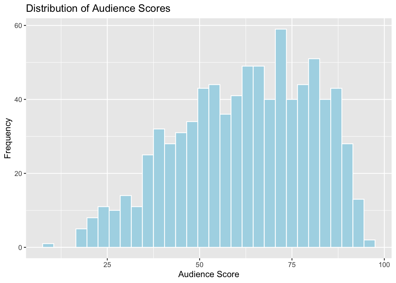
1.4.2 Density Plots
Density plots show the distribution for a quantitative variable like audience score. Scores can be compared across categories, like genre.
1.4.2.1 General Template for Density Plot
ggplot(data=DatasetName, aes(x=QuantitativeVariable,
                             color=CategoricalVariable, fill=CategoricalVariable)) +
  geom_density(alpha=0.2) +
  ggtitle("Plot Title") +
  xlab("Axis Label") +
ylab("Frequency") alpha, ranging from 0 to 1 dictates transparency.
1.4.2.2 Density Plot of Audience Scores
ggplot(data=MoviesSubset1, aes(x=AudienceScore, color=Genre, fill=Genre)) +
  geom_density(alpha=0.2) +
  ggtitle("Distribution of Audience Scores") +
  xlab("Audience Score") +
ylab("Frequency") 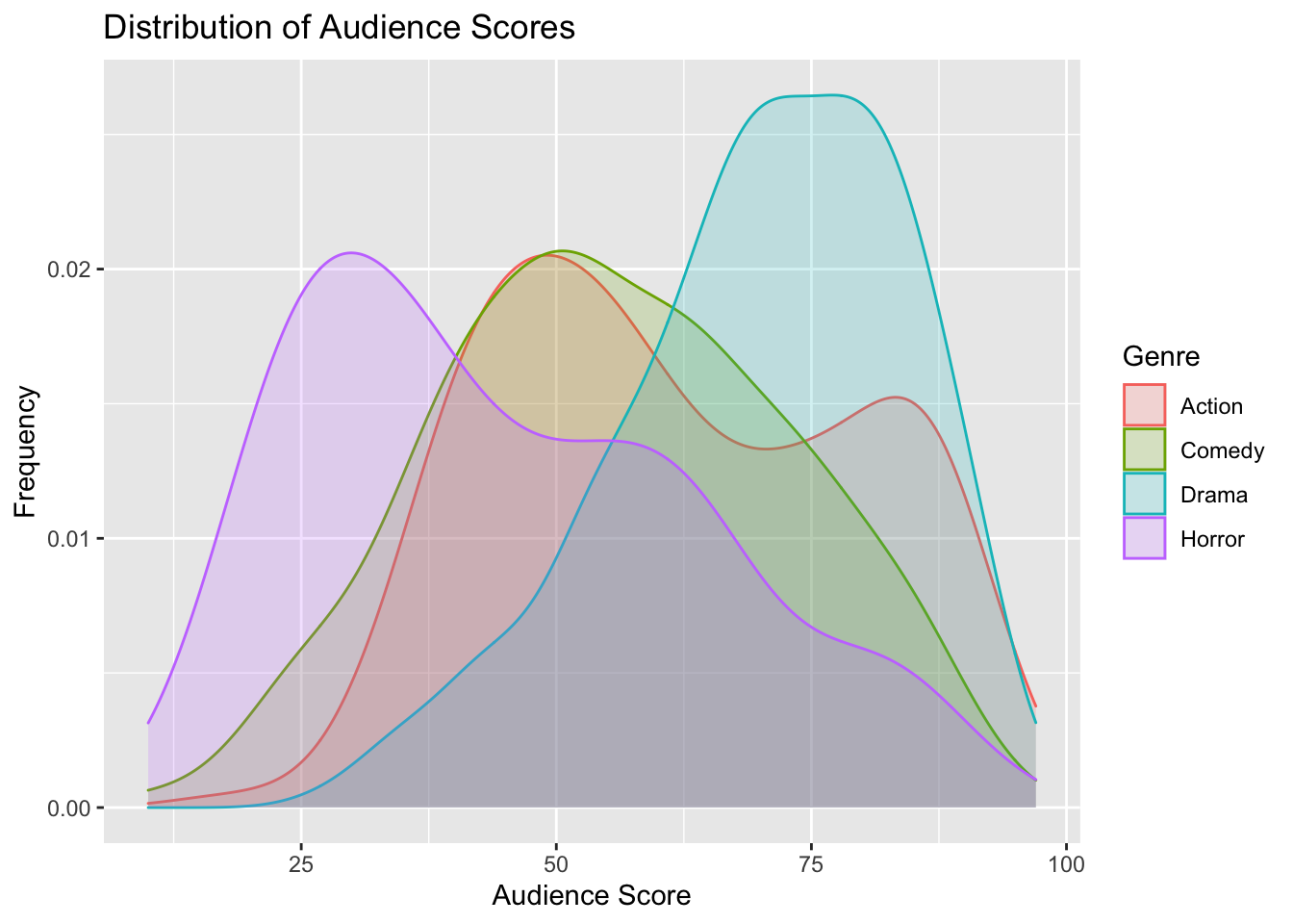
1.4.3 Boxplot
Boxplots can be used to compare a quantitative variable with a categorical variable
1.4.3.1 General Template for Boxplot
ggplot(data=DatasetName, aes(x=CategoricalVariable,
                             y=QuantitativeVariable)) +
  geom_boxplot() +
  ggtitle("Plot Title") +
  xlab("Variable Name") + ylab("Variable Name")
You can make the plot horizontal by adding + coordflip(). You can turn the axis text vertical by adding theme(axis.text.x = element_text(angle = 90)).
1.4.3.2 Boxplot Comparing Scores for Genres
ggplot(data=MoviesSubset1, aes(x=Genre, y=AudienceScore)) + geom_boxplot() +
  ggtitle("Audience Score by Genre") +
  xlab("Genre") + ylab("Audience Score") +
  theme(axis.text.x = element_text(angle = 90))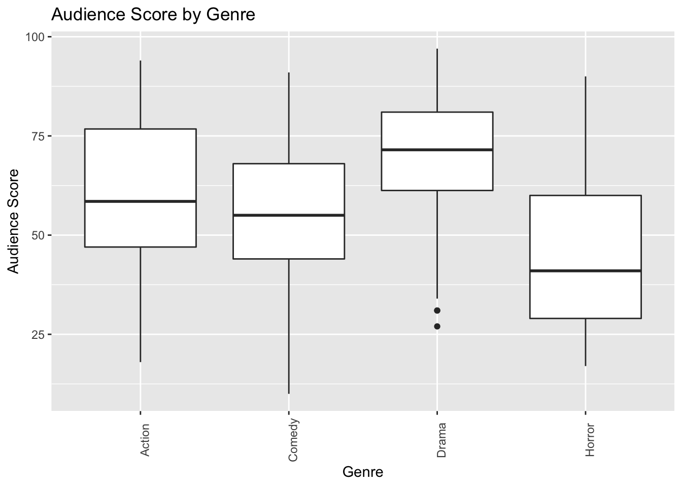
1.4.4 Violin Plot
Violin plots are an alternative to boxplots. The width of the violin tells us the density of observations in a given range.
1.4.4.1 General Template for Violin Plot
ggplot(data=DatasetName, aes(x=CategoricalVariable, y=QuantitativeVariable,
                             fill=CategoricalVariable)) +
  geom_violin() +
  ggtitle("Plot Title") +
  xlab("Variable Name") + ylab("Variable Name")
1.4.4.2 Violin Plot Comparing Scores for Genres
ggplot(data=MoviesSubset1, aes(x=Genre, y=AudienceScore, fill=Genre)) +
  geom_violin() +
  ggtitle("Audience Score by Genre") +
  xlab("Genre") + ylab("Audience Score") +
  theme(axis.text.x = element_text(angle = 90))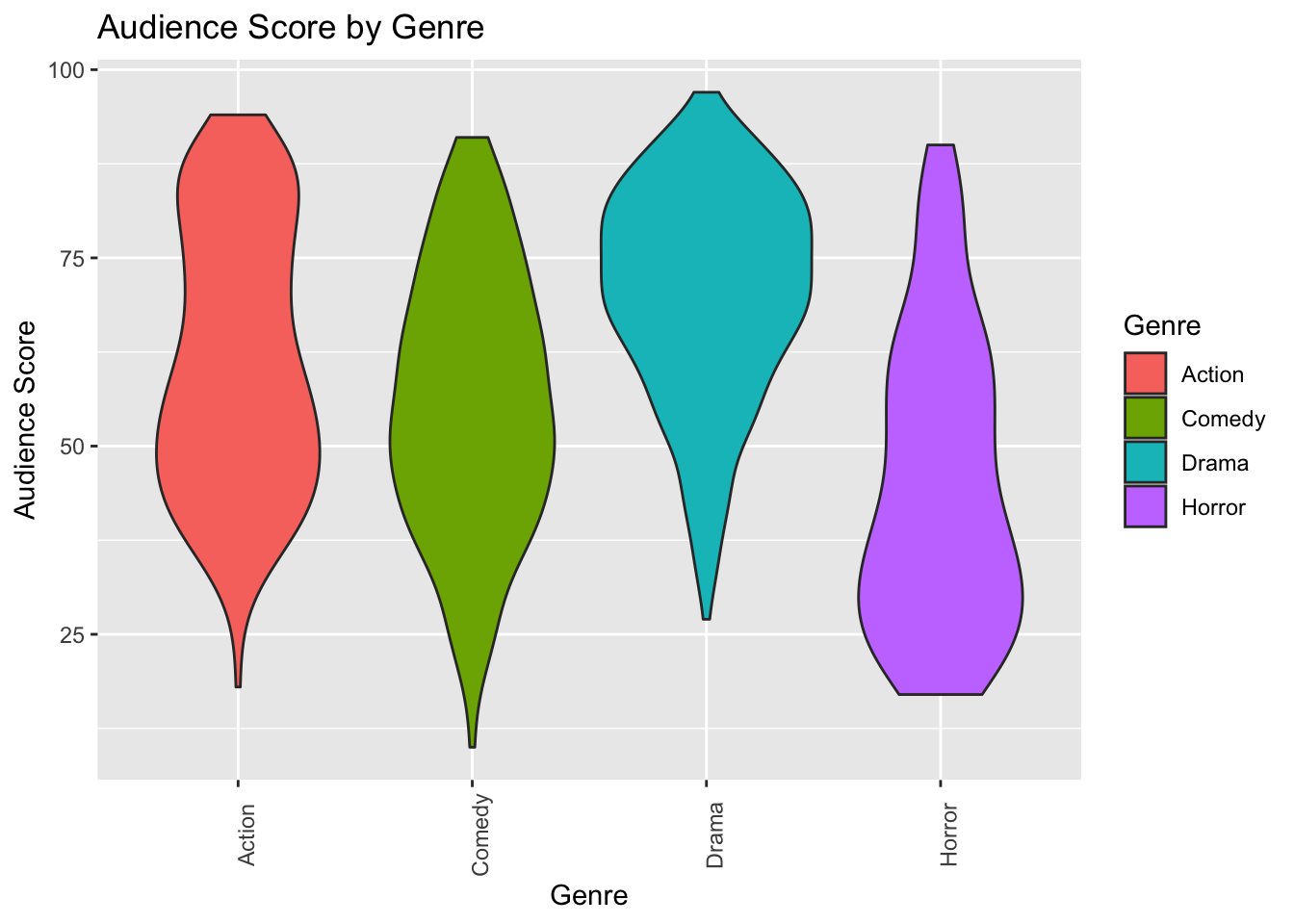
We can view the boxplot and violin plot together.
1.4.5 Scatterplots
Scatterplots are used to visualize the relationship between two quantitative variables.
1.4.5.1 Scatterplot Template
ggplot(data=DatasetName, aes(x=CategoricalVariable, y=QuantitativeVariable)) +
  geom_point() +
  ggtitle("Plot Title") +
  ylab("Axis Label") +
  xlab("Axis Label")
1.4.5.2 Scatterplot Comparing Audience Score and Rotten Tomatoes Score
ggplot(data=MoviesSubset1, aes(x=RottenTomatoes, y=AudienceScore)) +
  geom_point() +
  ggtitle("Audience and Critics Ratings") +
  ylab("Audience Rating") +
  xlab("Critics' Rating")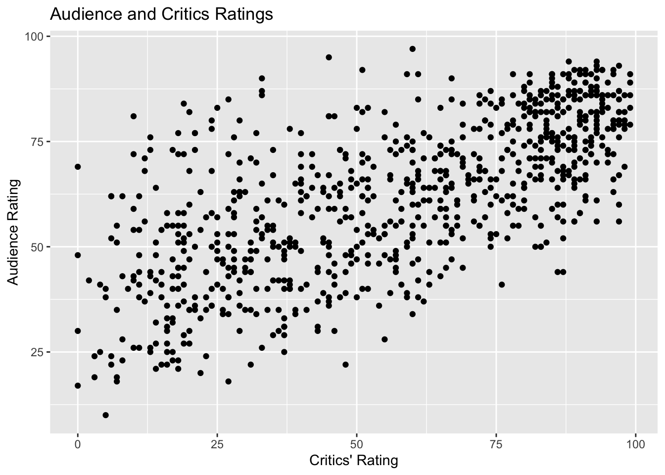
We see that there is an upward trend, indicating a positive association between critics scores (RottenTomatoes), and audience scores. However, there is a lot of variability, and the relationship is moderately strong at best.
We can also add color, size, and shape to the scatterplot to display information about other variables.
ggplot(data=MoviesSubset1,
       aes(x=RottenTomatoes, y=AudienceScore, color=Genre, size=WorldGross)) +
  geom_point() +
  ggtitle("Audience and Critics Ratings") +
  ylab("Audience Rating") +
  xlab("Critics' Rating")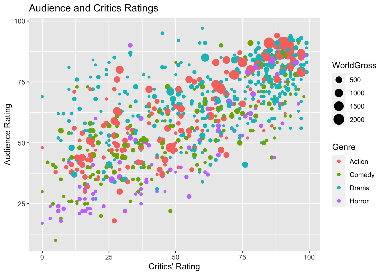
We can add labels for points meeting certain conditions, using geom_text(). This should be done carefully, to avoid overlap.
ggplot(data=MoviesSubset1,
       aes(x=RottenTomatoes, y=AudienceScore, color=Genre, size=WorldGross)) +
  geom_point() +
  ggtitle("Audience and Critics Ratings") +
  ylab("Audience Rating") + xlab("Critics' Rating") +
  geom_text(data = MoviesSubset1 %>% filter(WorldGross >800), aes(label = Movie),
            color="black", check_overlap = TRUE)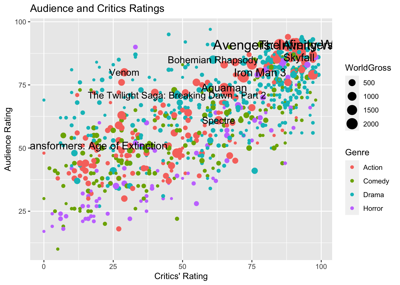
1.4.6 Bar Graphs
Bar graphs can be used to visualize one or more categorical variables
1.4.6.1 Bar Graph Template
ggplot(data=DatasetName, aes(x=CategoricalVariable)) +
  geom_bar(fill="colorchoice",color="colorchoice")  +
  ggtitle("Plot Title") +
  xlab("Variable Name") +
  ylab("Frequency")
1.4.6.2 Bar Graph by Genre
ggplot(data=MoviesSubset1, aes(x=Genre)) +
  geom_bar(fill="lightblue",color="white")  +
  ggtitle("Number of Films by Genre") +
  xlab("Genre") +
  ylab("Number of Films") +
  theme(axis.text.x = element_text(angle = 90))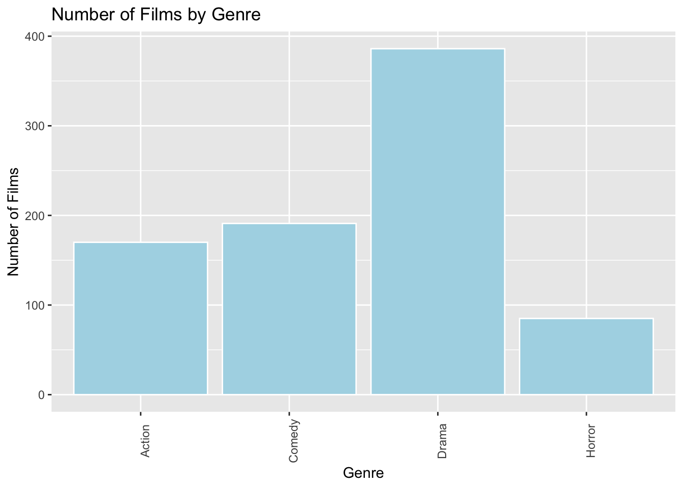
1.4.7 Stacked and Side-by-Side Bar Graphs
1.4.7.1 Stacked Bar Graph Template
ggplot(data = DatasetName, mapping = aes(x = CategoricalVariable1,
                                         fill = CategoricalVariable2)) +
    stat_count(position="fill")  +
  theme_bw() + ggtitle("Plot Title") +
  xlab("Variable 1") +
  ylab("Proportion of Variable 2") +
  theme(axis.text.x = element_text(angle = 90))
1.4.7.2 Stacked Bar Graph Example
The stat_count(position="fill") command creates a stacked bar graph, comparing two categorical variables. Let's explore whether certain genres are more profitable than others, using the profitability variable.
ggplot(data = MoviesSubset1, mapping = aes(x = Genre, fill = Profitable)) +
    stat_count(position="fill")  +
  theme_bw() + ggtitle("Profitability by Genre") +
  xlab("Genre") +
  ylab("Proportion Profitable") +
theme(axis.text.x = element_text(angle = 90)) 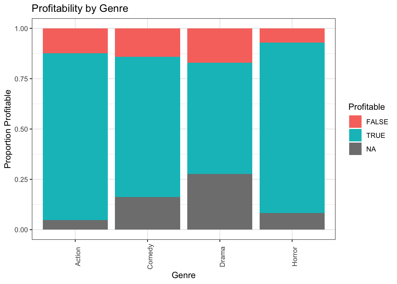
1.4.7.3 Side-by-side Bar Graph Template
We can create a side-by-side bar graph, using position=dodge.
ggplot(data = DatasetName, mapping = aes(x = CategoricalVariable1,
                                         fill = CategoricalVariable2)) +
    geom_bar(position = "dodge") +
  ggtitle("Plot Title") +
  xlab("Genre") +
  ylab("Frequency")
1.4.7.4 Side-by-side Bar Graph Example
ggplot(data = MoviesSubset1, mapping = aes(x = Genre, fill = Profitable)) +
    geom_bar(position = "dodge") +
  ggtitle("Number of Films by Genre") +
  xlab("Genre") +
  ylab("Number of Films") +
theme(axis.text.x = element_text(angle = 90)) 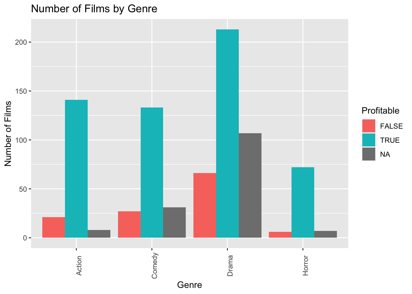
1.4.8 Examining Correlation
Correlation plots can be used to visualize relationships between quantitative variables. These can be helpful when we proceed to modeling. Explanatory variables that are highly correlated with the response are often strong predictors that should be included in a model. However, including two explanatory variables that are highly correlated with one another can create interpretation problems.
The cor() function calculates correlations between quantitative variables. We'll use select_if to select only numeric variables. The `use="complete.obs" command tells R to ignore observations with missing data.
1.4.8.1 Correlation Plot
cor(select_if(MoviesSubset1, is.numeric), use="complete.obs")## RottenTomatoes AudienceScore WorldGross Budget Year
## RottenTomatoes 1.000000000 0.71539895 0.13908396 -0.006259344 0.02860264
## AudienceScore 0.715398951 1.00000000 0.23150099 0.082716295 -0.04107899
## WorldGross 0.139083957 0.23150099 1.00000000 0.809560293 0.07300631
## Budget -0.006259344 0.08271629 0.80956029 1.000000000 0.03517844
## Year 0.028602637 -0.04107899 0.07300631 0.035178443 1.00000000The corrplot() function in the corrplot() package provides a visualization of the correlations. Larger, thicker circles indicate stronger correlations.
library(corrplot)
Corr <- cor(select_if(HollywoodMovies, is.numeric), use="complete.obs")
corrplot(Corr)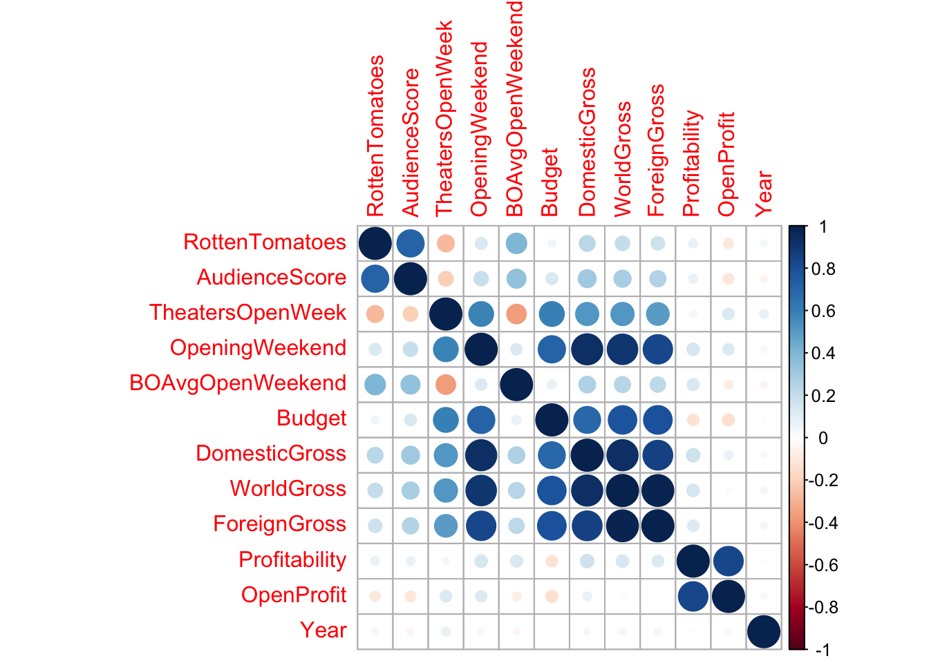
A scatterplot matrix is a grid of plots. It can be created using the ggpairs() function in the GGally package.
The scatterplot matrix shows us:
- Along the diagonal are density plots for quantitative variables, or bar graphs for categorical variables, showing the distribution of each variable.
- Under the diagonal are plots showing the relationships between the variables in the corresponding row and column. Scatterplots are used when both variables are quantitative, bar graphs are used when both variables are categorical, and boxplots are used when one variable is categorical, and the other is quantitative.
- Above the diagonal are correlations between quantitative variables.
We need to remove the column with the movie names. This is done using select.
1.4.8.2 Scatterplot Matrix
library(GGally)
ggpairs(MoviesSubset1 %>% select(-Movie))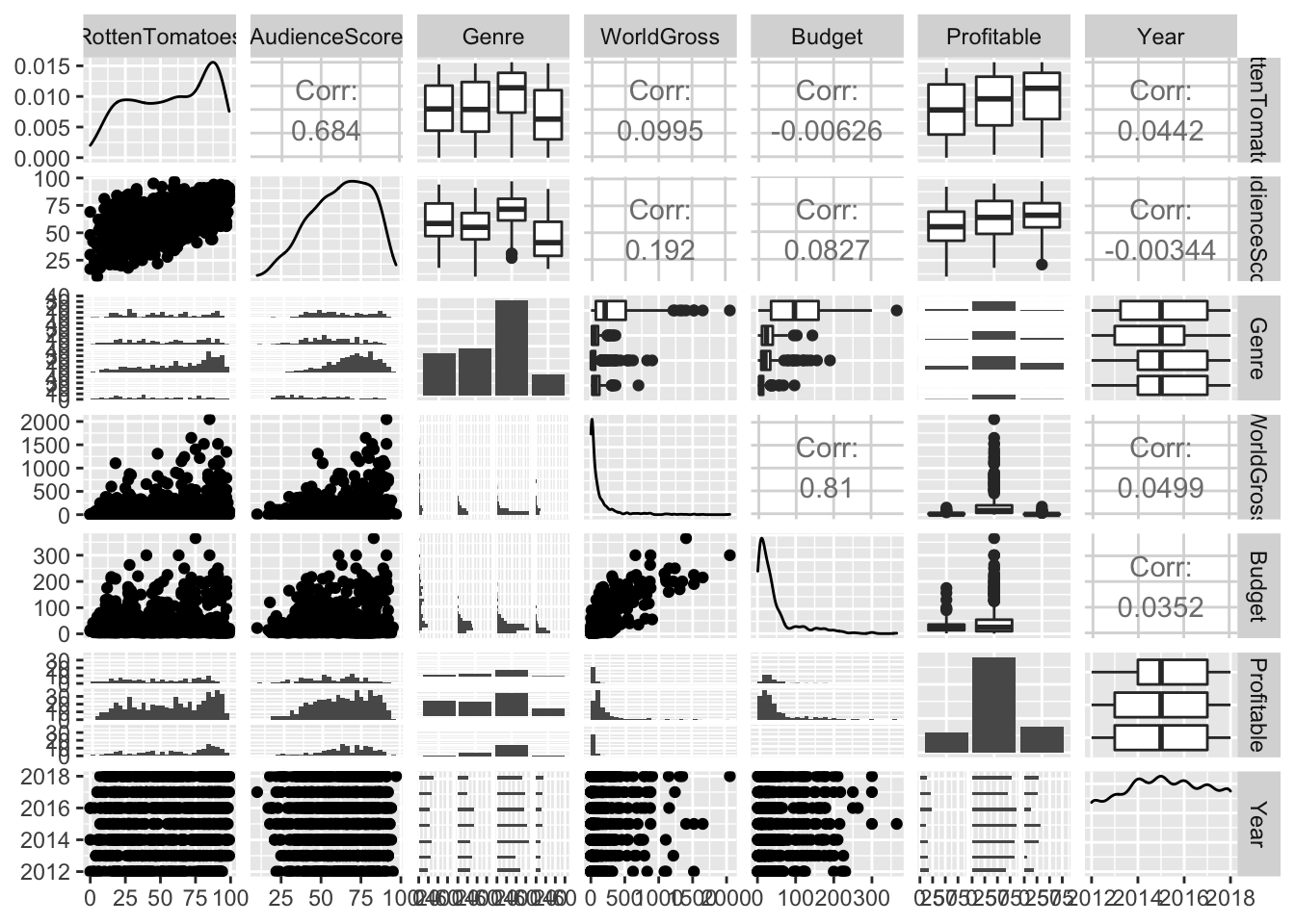
The scatterplot matrix is useful for helping us notice key trends in our data. However, the plot can hard to read as it is quite dense, especially when there are a large number of variables. These can help us look for trends from a distance, but we should then focus in on more specific plots.
1.5 Summary Tables
The group_by() and summarize() commands are useful for breaking categorical variables down by category. For example, let's calculate number of films in each genre, and the mean, median, and standard deviation in film WorldGross by genre.
Notes:
1. The n() command calculates the number of observations in a category.
2. The na.rm=TRUE command removes missing values, so that summary statistics can be calculated.
3. arrange(desc(Mean_Gross)) arranges the table in descending order of Mean_Gross. To arrange in ascending order, use arrange(Mean_Gross).
MoviesSubset1 %>% group_by(Genre) %>%
  summarize(N = n(),
            Mean_Gross = mean(WorldGross, na.rm=TRUE),
            Median_Gross = median(WorldGross, na.rm=TRUE),
            StDev_Gross = sd(WorldGross, na.rm = TRUE)) %>%
  arrange(desc(Mean_Gross))
## # A tibble: 4 x 5
## Genre N Mean_Gross Median_Gross StDev_Gross
## <chr> <int> <dbl> <dbl> <dbl>
## 1 Action 170 355. 211. 391.
## 2 Horror 85 95.7 62.2 111.
## 3 Comedy 191 74.5 47.5 75.0
## 4 Drama 386 58.1 20.6 106.The kable() function in the knitr() package creates tables with professional appearance.
library(knitr)
MoviesTable <- MoviesSubset1 %>% group_by(Genre) %>%
  summarize(N = n(),
            Mean_Gross = mean(WorldGross, na.rm=TRUE),
            Median_Gross = median(WorldGross, na.rm=TRUE),
            StDev_Gross = sd(WorldGross, na.rm = TRUE)) %>%
  arrange(desc(Mean_Gross))
kable(MoviesTable)| Genre | N | Mean_Gross | Median_Gross | StDev_Gross |
|---|---|---|---|---|
| Action | 170 | 354.58253 | 210.66 | 390.75176 |
| Horror | 85 | 95.73859 | 62.19 | 110.82866 |
| Comedy | 191 | 74.48487 | 47.51 | 75.01561 |
| Drama | 386 | 58.12212 | 20.60 | 105.74866 |