Chapter 7 Simulation-based Inference
The type of inference you will perform depends on the type of data you are analyzing.
response variable (def) is the variable we think is being impacted or changed by the explanatory variable.
explanatory variable (def) is the variable we think is “explaining” the change in the response variable.
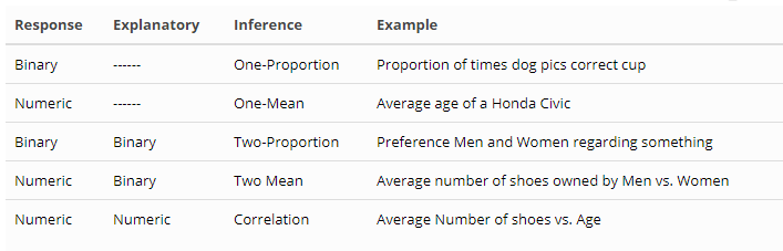
Here are the 7 general steps to performing an inference procedure using simulation techniques:
| Step |
|---|
|
|
|
|
|
|
|
7.1 One-Proportion Inference
| Step | Example |
|---|---|
|
Less than 50% of New York City Voters will support some policy |
|
1000 voters in NYC |
|
Let pi be the proportion of NYC voters who support the policy. H0: pi = 0.50; Ha: pi < 0.50 |
|
p-hat = 460/1000, or 46% |
|
Simulate a one-proportion inference n = 1000, observed = 460 |
|
One-sided p-value = 0.002 |
|
Since the p-value is so small, we reject the null hypothesis and we have evidence to believe that less than 50% of NYC voters support the policy |
7.1.1 When do we use one-proportion inference?
When we want to test the claim that a population proportion is not equal to some fixed percentage. For example, the proportion of women within some church congregation is greater than 55%.
\(H_0: \pi = 0.55\)
\(H_a: \pi > 0.55\)
Test statistic: we use the observed proportion from the sample. In this case, we identify a sample of church members and count how many women there are. Let’s say there are 62 out of 100. We say \(\hat{p} = 0.62\)
Let’s develop an algorithm using simulation to replicate the One-Proportion applet found at link.
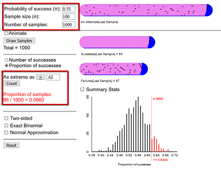
We will test the above claim that the proportion of women in the church congregation is greater than 55% by simulating a large number of trials of flipping n coins:
pi <- 0.55   # probability of success for each toss
n <- 100   # Number of times we toss the penny (sample size)
trials <- 1000   # Number of trials (number of samples)

observed <- 62  # Observed number of heads

phat = observed / n   # p-hat - the observed proportion of heads

data.sim <- do(trials) * rflip(n, prob = pi )

head(data.sim)
## n heads tails prop
## 1 100 62 38 0.62
## 2 100 53 47 0.53
## 3 100 50 50 0.50
## 4 100 44 56 0.44
## 5 100 54 46 0.54
## 6 100 50 50 0.50If we consider the above distribution to be our null distribution, we can now consider the likelihood that we would observe a value “as extreme as” our test statistic - 62 heads in this case.
histogram(~prop, data = data.sim,
          v = phat,
          width = 0.025,
          xlab = "Proportion of women",
          main = "Null hypothesis distribution",
groups = prop >= phat) 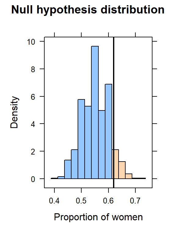
To compute a p-value, we simply need to count the number of times, in our null distribution, we observed a value as extreme (or more so) as the test statistic, p-hat.
if(observed > pi * n) {
  pvalue <- sum(data.sim$prop >= phat) / trials
} else {
  pvalue <- sum(data.sim$prop <= phat) / trials
}

paste("One-sided p-value is", pvalue)
## [1] "One-sided p-value is 0.095"paste("Two-sided p-value is", 2 * pvalue)## [1] "Two-sided p-value is 0.19"Conclusion: if the p-value is less than the level of significance, we REJECT H0 and conclude that there is evidence to support the alternative. In this case, we have a rather large p-value (0.095), so we FAIL TO REJECT H0. There is not evidence to support the above claim.
7.1.2 One-Proportion Inference Code
library(mosaic)

pi <- 0.55   # probability of success for each toss
n <- 100   # Number of times we toss the penny (sample size)
trials <- 1000   # Number of trials (number of samples)

observed <- 62  # Observed number of heads

phat = observed / n   # p-hat - the observed proportion of heads

data.sim <- do(trials) * rflip(n, prob = pi )

histogram(~prop, data = data.sim,
          v = phat,
          width = 0.025,
          xlab = "Proportion",
          main = "Null hypothesis distribution",
          groups = prop >= phat)

if(observed > pi * n) {
  pvalue <- sum(data.sim$prop >= phat) / trials
} else {
  pvalue <- sum(data.sim$prop <= phat) / trials
}

paste("One-sided p-value is", pvalue)
paste("Two-sided p-value is", 2 * pvalue)
7.2 One-Mean Inference
Here is the procedure for using a Confidence Interval to analyze a single mean.
| Step | Example |
|---|---|
|
According to a 2000 report, the average number of flip-flops owned by a typical college student in the US is 3 |
|
A bunch of students in a data science class |
|
Let mu be the average number of flip-flops owned by a college student. H0: mu = 3; Ha: mu > 3 |
|
x-bar (sample mean) = 5.26 |
|
Simulate a one-mean inference, 95% confidence interval is (4.3, 6.32) |
|
Since our sample mean falls within the interval, it is a plausible value for mu |
|
We fail to reject the null hypothesis and do not have evidence to believe that the number of flip-flops owned by a typical college student is greater than 3. |
| Step | Example |
|---|---|
|
According to a 2000 report, the average number of flip-flops owned by a typical college student in the US is 3 |
|
A bunch of students in a data science class |
|
Let mu be the average number of flip-flops owned by a college student. H0: mu = 3; Ha: mu > 3 |
|
x-bar (sample mean) = 5.26 |
|
Simulate a one-mean inference |
|
p-value = 0.0165 |
|
We reject the null hypothesis and have evidence to believe that the number of flip-flops owned by a typical college student is greater than 3. |
7.2.1 When do we use one-mean inference?
When we want to test the claim that a population mean is not equal to some fixed value. For example, the average miles-per-gallon of a car is equal to 22.
\(H_0: \mu = 22\) \(H_a: \mu \ne 22\)
Test statistic: we use the observed mean from the sample. In this case, we will compute the mean of the mtcars data \(\bar{x} = 20.09\)
mu = 22

favstats(~mpg, data=mtcars)
## min Q1 median Q3 max mean sd n missing
## 10.4 15.425 19.2 22.8 33.9 20.09062 6.026948 32 0observed <- mean(~mpg, data=mtcars, na.rm=T)
paste("Observed value for sample mean: ", observed)## [1] "Observed value for sample mean: 20.090625"Let’s develop an algorithm using simulation to compute a confidence interval for a single mean, using simulation. we will use the resample() function to create a null distribution from the sample.
trials <- 1000
samples <- do(trials) * mosaic::mean(~mpg, data=resample(mtcars))
# Let's compute a 95% Confidence Interval
(ci <- quantile(samples$mean,c(0.025,0.975))) ## 2.5% 97.5%
## 18.07781 22.13758Interpretation: We are 95% confident that the population mean is within the interval (17.45, 22.99). Since the test statistic of 22 is within this interval, we FAIL TO REJECT the claim that the average miles per gallon of all cars is not equal to 22 mpg.
And we can look at the distribution of sample means for our resampled data.
histogram(~mean, data=samples,
main = "Distribution of sample means",
v = c(ci[1], ci[2])
)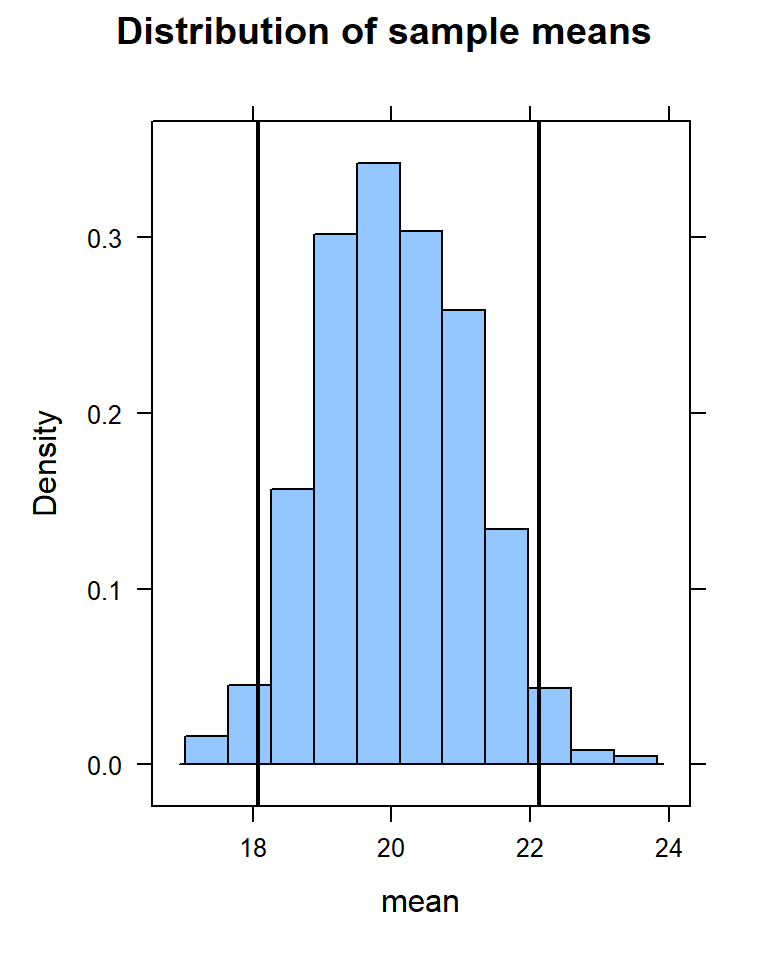 Notice that the value of 22 falls just within the confidence interval.
Let’s compute the p-value.
if(observed < mu) {
pvalue <- sum(samples$mean >= mu) / trials
} else {
pvalue <- sum(samples$mean <= mu) / trials
}
paste("One-sided p-value is", pvalue)## [1] "One-sided p-value is 0.035"paste("Two-sided p-value is", 2 * pvalue)## [1] "Two-sided p-value is 0.07"Since this is a two-sided test of inference (mpg not equal to 22), we fail to reject the null hypothesis. We do not have evidence to believe that the mpg of all cars is different from 22 mile-per-gallon.
7.2.2 One-mean Inference Code
library(mosaic)
# Read your data here
mu = 22
favstats(~mpg, data=mtcars)
observed <- mean(~mpg, data=mtcars, na.rm=T)
paste("Observed value for sample mean: ", observed)
trials <- 1000
samples <- do(trials) * mosaic::mean(~mpg, data=resample(mtcars))

# Let's compute a 95% Confidence Interval
(ci <- quantile(samples$mean,c(0.025,0.975)))
histogram(~mean, data=samples,
          main = "Distribution of sample means",
          v = c(ci[1], ci[2])
          )
if(observed < mu) {
  pvalue <- sum(samples$mean >= mu) / trials
} else {
  pvalue <- sum(samples$mean <= mu) / trials
}

paste("One-sided p-value is", pvalue)
paste("Two-sided p-value is", 2 * pvalue)7.3 Two-proportion inference
| Step | Example |
|---|---|
|
The death rate on Nurse Gilbert’s shifts is higher than the base death rate |
|
all shifts in the hospital |
|
Let pi1 be the proportion of patients who die on Nurse Gilbert shifts; pi2 will be the proportion of patients who die on shifts when Nurse Gilbert does not work. H0: pi1 = pi2; Ha: pi1 > pi2 |
|
p-hat1 = 0.156; p-hat2 = 0.025 |
|
Simulate a two-proportion inference n = 1000 |
|
One-sided p-value = 0 |
|
Since the p-value is so small, we reject the null hypothesis and we have evidence to believe that the death rate on Nurse Gilbert shifts is higher than the death rate on shifts when Nurse Gilbert does not work. |
7.3.1 When do we use two-proportion inference?
When we want to test the claim that two population proportions are significantly different. For example, the proportion of women who are in favor of some policy vs. the proportion of men who are in favor of the policy.
Let \(\pi_1\) be the proportion of women who favor the policy
Let \(\pi_2\) be the proportion of men who favor the policy
\(H_0: \pi_1 = \pi_2\) \(H_a: \pi_1 \ne \pi_2\)
Test statistic: we use the observed proportions from the sample. In this case, we identify a sample of church members, determine their gender, and ask them if they support the policy. Let’s say that out of 100 women, 62 support the policy, giving us \(\hat{p}_1 = 0.62\), and out of 100 men, 51 support the policy, giving us \(\hat{p}_2 = 0.51\).
Let’s develop an algorithm using simulation to replicate the Two-Proportion applet found at link.
First, we need to create a dataframe representing the individual subjects in the study. We know the summary information that 51% of the men and 62% of the women support the policy. We will need to create, in effect 200 rows representing each of the subjects, as follows:
# Step 1:  Create a dataframe representing the two variables
# NOTE:  Values should be in alphabetical order
# df <- data.table(Group = c(rep("men", 100),
              #              rep("women", 100)),
              # Support = c(rep("no",38),
              #             rep("yes", 62),
              #             rep("no",49),
              #             rep("yes",51)))

df <- rbind(
  do(38) * data.frame(Group = "Men", Support = "no"),
  do(62) * data.frame(Group = "Men", Support = "yes"),
  do(49) * data.frame(Group = "Women", Support ="no"),
  do(51) * data.frame(Group = "Women", Support = "yes")
)

# Compute my summary AND print the results
(df.summary <- tally(Support ~ Group, data=df))
## Group
## Support Men Women
## no 38 49
## yes 62 51tally(Support~Group, data=df, format="proportion")## Group
## Support Men Women
## no 0.38 0.49
## yes 0.62 0.5162% of the men support the policy and 51% of the women support the policy.
Let’s compute the difference in the two sample proportions, and view a barplot of the data:
# Step 2:  Compute the observed difference in proportions
observed <- diffprop(Support ~ Group, data = df)
paste("Observed difference in proportions: " , round(observed,3))
## [1] "Observed difference in proportions: 0.11"barplot(prop.table(df.summary, margin = 2),
las = 1,
main = "Proportion that Support",
col = c("green", "purple"),
legend.text = c("no", "yes"))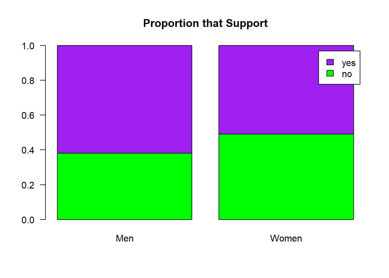
Let’s shuffle the treatment labels and look at the null distribution.
# STep 3: Shuffle the treatment labels
trials <- 1000
null.dist <- do(trials) * diffprop(Support ~ shuffle(Group), data=df)
histogram( ~ diffprop, data= null.dist,
xlab = "Differences in proportions",
main = "Null distribution for differences in proportions",
v= observed)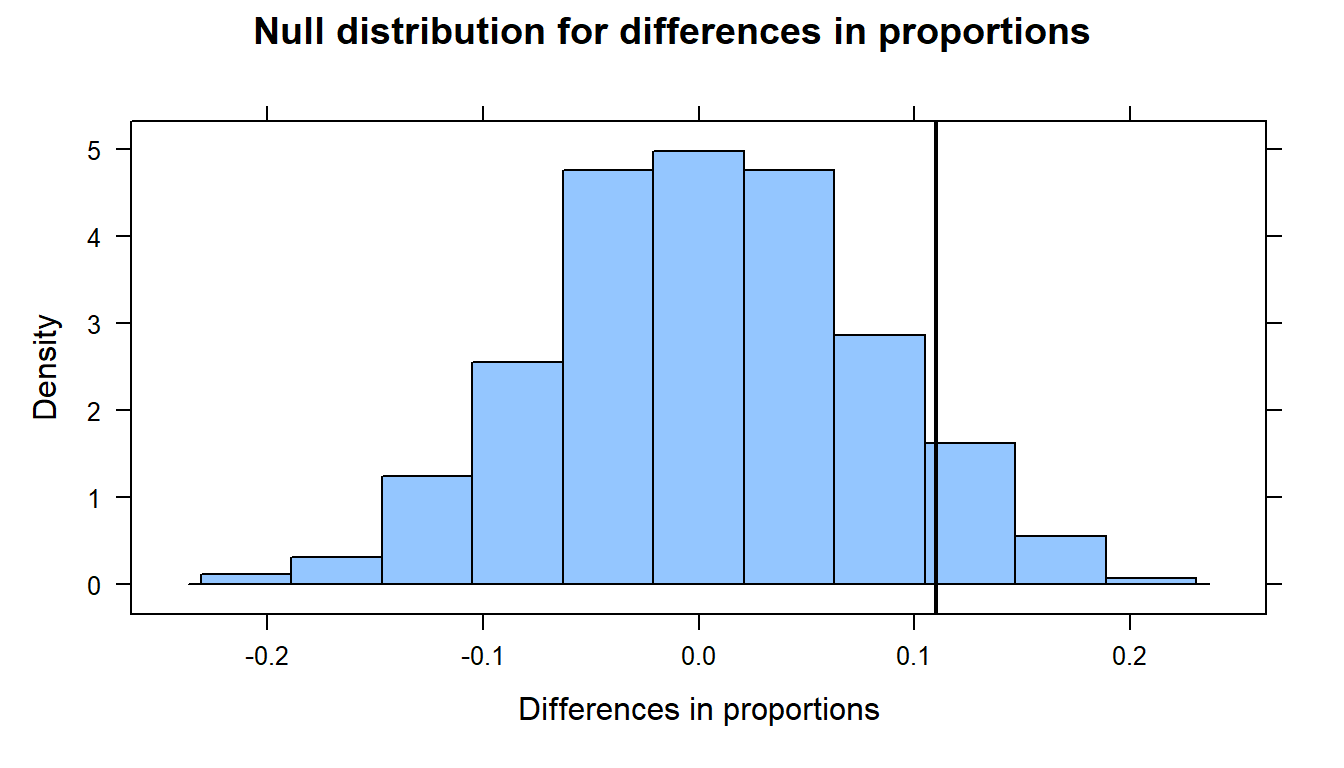
Lastly, we’ll compute the p-value - that is, the probability of observing a test statistic as extreme (or more so) as 0.11, given that the null hypothesis is true.
if (observed > 0 ) {
p.value <- prop(~diffprop >= observed, data= null.dist)
} else {
p.value <- prop(~diffprop <= observed, data= null.dist)
}
paste(" One-sided p-value: ", round(p.value,3))## [1] " One-sided p-value: 0.094"paste(" Two-sided p-value: ", 2 * round(p.value,3))## [1] " Two-sided p-value: 0.188"7.3.2 Two-Proportion Inference Code - Method I (rbind):
library(mosaic)
library(data.table)
# Step 1: Create a dataframe representing the two variables
# NOTE: Values should be in alphabetical order
df <- rbind(
do(38) * data.frame(Group = "Men", Support = "no"),
do(62) * data.frame(Group = "Men", Support = "yes"),
do(49) * data.frame(Group = "Women", Support ="no"),
do(51) * data.frame(Group = "Women", Support = "yes")
)
# Compute my summary AND print the results
(df.summary <- tally(Support ~ Group, data=df))
tally(Support~Group, data=df, format="proportion")
# Step 2: Compute the observed difference in proportions
observed <- diffprop(Support ~ Group, data = df)
paste("Observed difference in proportions: " , round(observed,3))
barplot(prop.table(df.summary, margin = 2),
        las = 1,
        main = "Proportion that Support",
        col = c("green", "purple"),
        legend.text = c("no", "yes"))
# STep 3: Shuffle the treatment labels
trials <- 1000
null.dist <- do(trials) * diffprop(Support ~ shuffle(Group), data=df)
histogram( ~ diffprop, data= null.dist,
xlab = "Differences in proportions",
main = "Null distribution for differences in proportions",
groups= diffprop >= observed,
v= observed)
if (observed > 0 ) {
p.value <- prop(~diffprop >= observed, data= null.dist)
} else {
p.value <- prop(~diffprop <= observed, data= null.dist)
}
paste("One-sided p-value is", pvalue)
paste("Two-sided p-value is", 2 * pvalue)7.3.3 Two-Proportion Inference Code - Method II (matrix):
library(mosaic)
library(data.table)
rm(list=ls())

# Step 1:  Create a dataframe representing the two variables
df <- matrix(c(15,3,4,8), nrow = 2)
rownames(df) <- c("Positive", "Negative")
colnames(df) <- c("Good", "Bad")

# Step 2: Compute our differences
total_col1 <- sum(df[,1])
prop_col1 <- df[1,1]/total_col1
total_col2 <- sum(df[,2])
prop_col2 <-  df[1,2]/total_col2

observed <- prop_col1 - prop_col2
paste("Proportion - column 1: " , round(prop_col1,3))
paste("Proportion - column 2: " , round(prop_col2,3))
paste("Observed difference in proportions: " , round(observed,3))
paste("Relative Risk: " , round(prop_col1/prop_col2,3))

barplot(prop.table(df,margin = 2),
        las = 1,
        main = "xxxxxxx",
        ylab = "Observed proportion",
        col = c("green", "purple"),
        legend.text = rownames(df))

# STep 3:  Shuffle the treatment labels and compute a p-value
trials <- 1000
null.dist <- do(trials) * (mean(sample(0:1, total_col1, replace = T)) -
                             mean(sample(0:1, total_col2, replace=T)))

histogram( ~ result, data= null.dist,
           xlab = "Differences in proportions",
           main = "Null distribution for differences in proportions",
           v= observed)

if (observed > 0) {
  p.value <- prop(~result >= observed, data= null.dist)
} else {
  p.value <- prop(~result <= observed, data= null.dist)
}

paste(" One-sided p-value:  ", round(p.value,3))
paste(" Two-sided p-value:  ", 2 * round(p.value,3))
7.4 Two-mean inference
| Step | Example |
|---|---|
|
Inter-eruption times by Old Faithful changed between 1978 and 2003 |
|
the 203 observations made in which we measured the inter-eruption times |
|
Let mu1 be the inter-eruption time in 1978; mu2 is the inter-eruption time in 2003. H0: mu1 = mu2; Ha: mu1 not = mu2 |
|
x-bar1 = 71.07 minutes; x-bar2 = 91.19 minutes |
|
Simulate a two-mean inference assuming the times are equal |
|
One-sided p-value = 0 |
|
Since the p-value is so small, we reject the null hypothesis and we have evidence to believe that the inter-eruption times are different in 2003 from 1978. |
When do we use two-mean inference?
When we want to test the claim that two population means are significantly different. For example, the average amount of mercury found in two types of tuna fish - albacore and yellowfin
Let \(\mu_1\) be the average amount of mercury in albacore Let \(\mu_2\) be the average amount of mercury in yellowfin
\(H_0: \mu_1 = \mu_2\) \(H_a: \mu_1 \ne \mu_2\)
Test statistic: we use the observed sample means. We will have to compute these from the data.
Let’s read in the data and compute the sample means
read.delim("http://citadel.sjfc.edu/faculty/ageraci/data/tuna.txt") -> df
str(df)
## 'data.frame': 274 obs. of 2 variables:
## $ Tuna : chr "albacore " "albacore " "albacore " "albacore " ...
## $ Mercury: num 0 0.41 0.82 0.32 0.036 0.28 0.29 0.34 0.36 0.42 ...options(digits = 5)
favstats(~Mercury | Tuna, data=df)## Tuna min Q1 median Q3 max mean sd n missing
## 1 albacore 0 0.300 0.3600 0.3965 0.820 0.35763 0.13799 43 0
## 2 yellowfin 0 0.184 0.3109 0.4625 1.478 0.35444 0.23100 231 0Now we will compute the observed difference in the means:
# Compute the observed difference in the means between the two groups
observed <- diffmean(~Mercury | Tuna, data=df, na.rm = T)
paste("Observed difference in the means: ", round(observed, 3 ))
## [1] "Observed difference in the means: -0.003"Next we will ‘shuffle()’ the Tuna variable and compare the means:
trials <- 1000
moreorless <- "less"

# Compare the difference in means when we shuffle the Tuna varaible - do this lots of times
null.dist <- do(trials) * diffmean(Mercury ~ shuffle(Tuna), data=df, na.rm = T)

# Graph the histogram with the observed difference of proportions
histogram( ~ diffmean, data=null.dist,
           main = "Sampling distribution for null hypothesis",
           xlab = "Difference in means",
           v = observed, na.rm = T)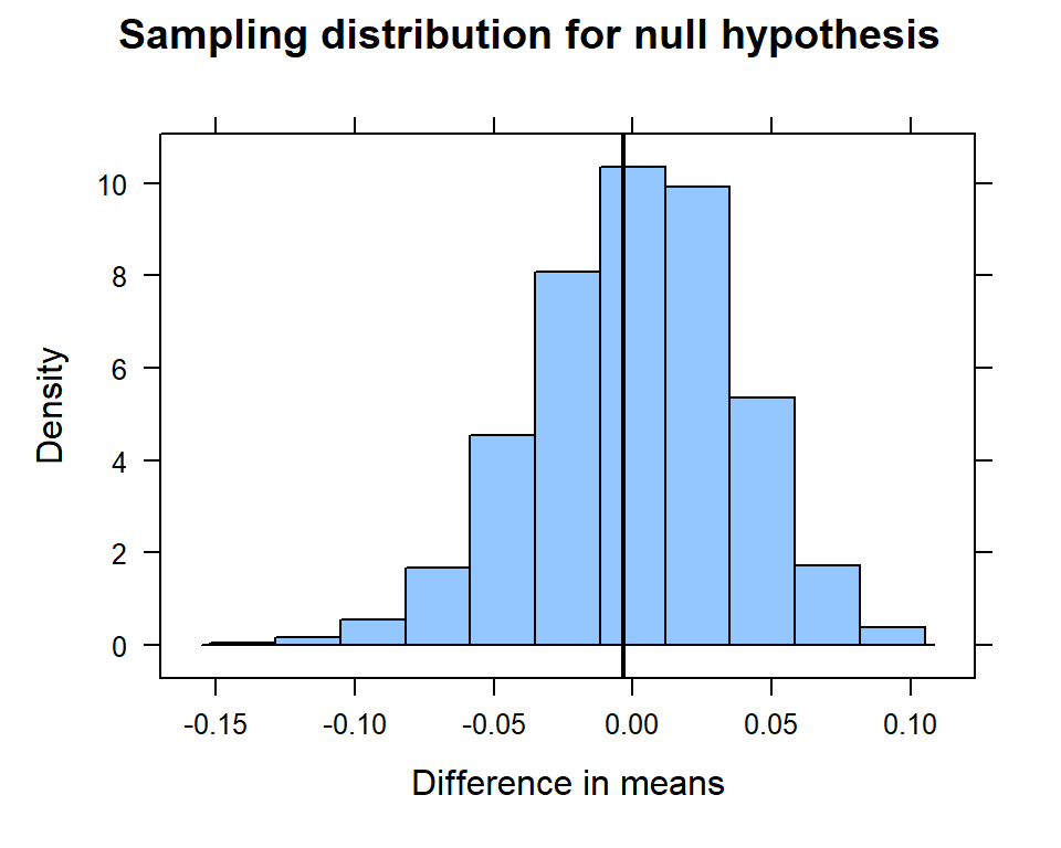
… and compute the p-value.
# Let's compute the p-value
if (moreorless == "more") {
  pvalue <- prop(~ diffmean >= observed, data=null.dist)
} else {
  pvalue <- prop(~ diffmean <= observed, data=null.dist)
}
paste("The one-sided p-value is ", round(pvalue,3))
## [1] "The one-sided p-value is 0.432"paste("The two-sided p-value is ", 2 * round(pvalue,3))## [1] "The two-sided p-value is 0.864"7.4.1 Two-Mean Inference Code:
library(mosaic)
library(data.table)
df <- read.delim("http://citadel.sjfc.edu/faculty/ageraci/data/tuna.txt")

favstats(~Mercury | Tuna, data=df)

# Compute the observed difference in the means between the two groups
observed <- diffmean(~Mercury | Tuna, data=df, na.rm = T)
paste("Observed difference in the means: ", round(observed, 3 ))

trials <- 1000

# Compare the difference in means when we shuffle the Tuna varaible - do this lots of times
null.dist <- do(trials) * diffmean(Mercury ~ shuffle(Tuna), data=df, na.rm = T)

# Graph the histogram with the observed difference of proportions
histogram( ~ diffmean, data=null.dist,
           main = "Sampling distribution for null hypothesis",
           xlab = "Difference in means",
           groups = diffmean >= observed,
           v = observed, na.rm = T)

# Let's compute the p-value
if (observed > 0) {
  pvalue <- prop(~ diffmean >= observed, data=null.dist)
} else {
  pvalue <- prop(~ diffmean <= observed, data=null.dist)
}
paste("The one-sided p-value is ", round(pvalue,3))
paste("The two-sided p-value is ", 2 * round(pvalue,3))