Chapter 6 Data Visualization

One of the strengths of R is the relative ease in which one can produce a nice looking graph. We will again use the formula template for making a graph:

plotname(~variable, data = dataName)

As you can see, there are three pieces of information we must provide to get the graph we want:

The kind of plot (histogram(), bargraph(), bwplot(), etc)
The name of the variable(s)
The name of the dataframe

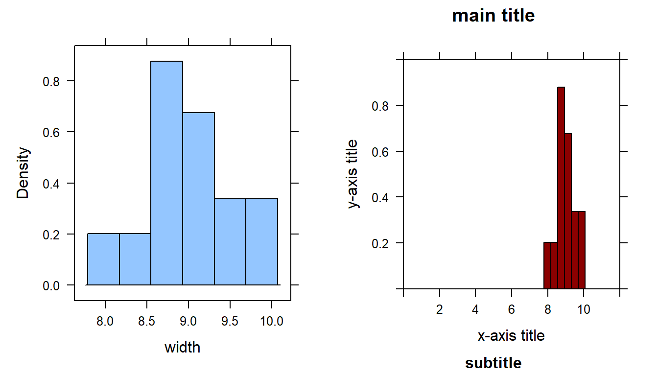
For example, let’s look at a basic histogram:

library(mosaic)

histogram(~width, data=KidsFeet)

histogram(~width, data=KidsFeet, 
          main = "main title",
          xlab = "x-axis title", 
          xlim = c(min, max), 
          ylab = "y-axis title", 
          ylib = c(min,max), 
          sub = "subtitle", 
          col = "dark red")

We can control the appearance of the graph using the following options:

main = title at top of graph
xlab = x-axis label
xlim = minimum/maximum of limits on x-axis
ylab = y-axis label
ylim = minimum/maximum of limits on y-axis
sub = subtitle
col or fcol = color of filled portion of graph (use fcol if data is in groups)

6.1 bargraphs - for one or two catagorical variables

A bargraph is used to display COUNTS for the number of observations in a datafile within certain categories. For example, let’s say we want to view the number of children in each of the boy/girl categories, or the right/left hand categories.

library(mosaic)

bargraph(~sex, data=KidsFeet, main = "sex")
bargraph(~domhand, data=KidsFeet, main = "dominant hand")

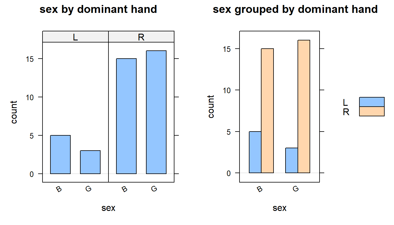
bargraph(~sex |domhand, data=KidsFeet, main = "sex by dominant hand")
bargraph(~sex,  groups=domhand, data=KidsFeet, main = "sex grouped by dominant hand")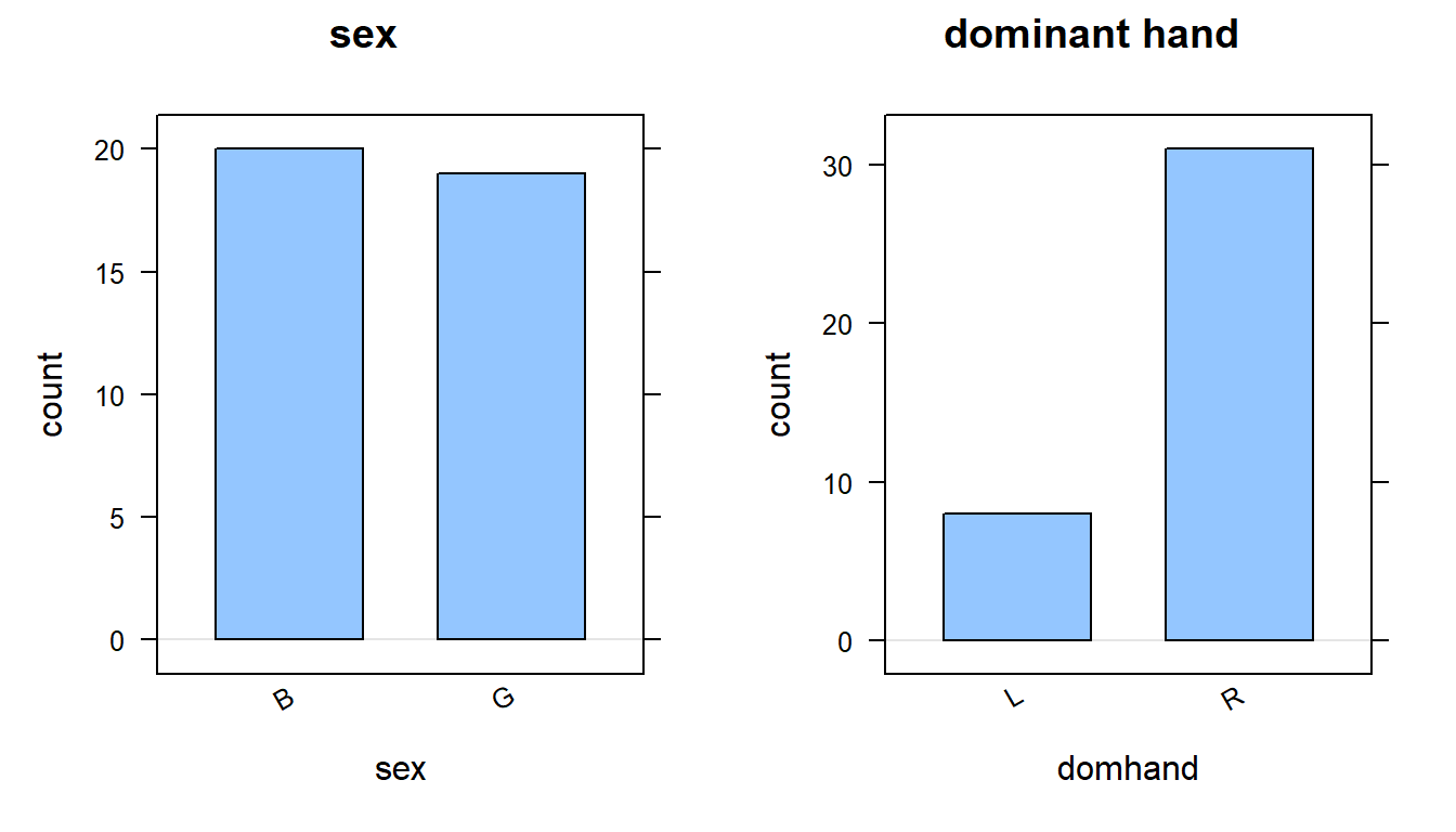

What about with summarized data?

df2 <-data.frame(twoparent =c(407,45), 
                 always =c(61,16), 
                 divorce =c(231,29),
                 nocohab =c(124,11),
                 withcohab =c(193,51),
                 row.names =c("yes", "no"))

df2

##     twoparent always divorce nocohab withcohab
## yes       407     61     231     124       193
## no         45     16      29      11        51

barplot(as.matrix(df2), legend.text =T, col =c("purple","magenta"))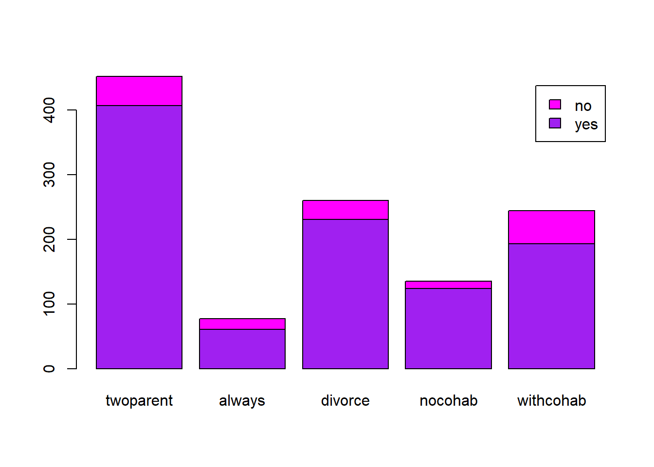

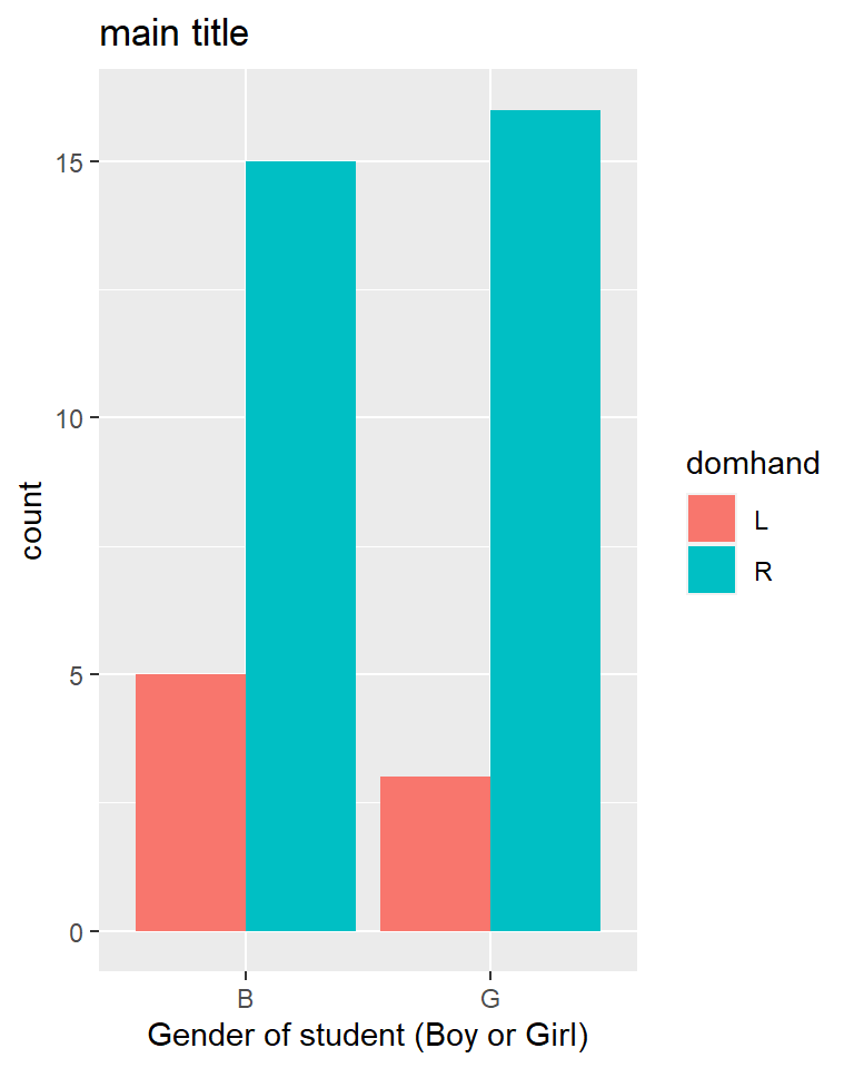
6.2 gf_bargraph - for categorical data

Note the the gf_bargraph() function uses title= instead of main= for the title of the graph.

library(ggformula)
gf_bar(~sex, fill = ~ domhand,   data=KidsFeet, 
       title = "main title",
       xlab = "Gender of student (Boy or Girl)",
       position = position_dodge())

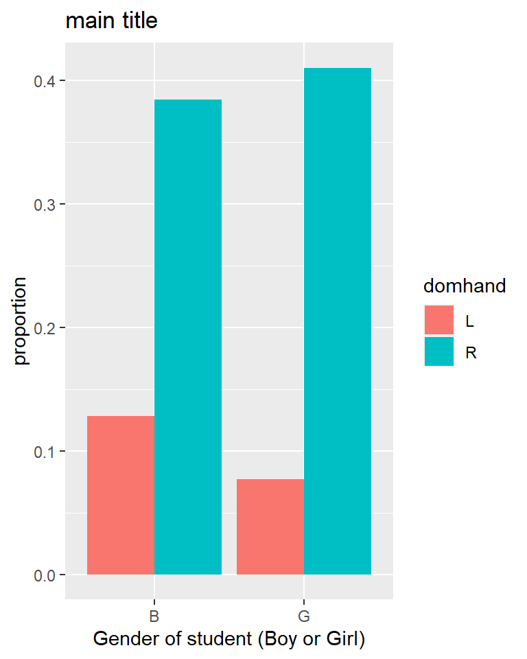
gf_props(~sex, fill = ~ domhand,   data=KidsFeet, 
       title = "main title",
       xlab = "Gender of student (Boy or Girl)",
       position = position_dodge())

gf_bar() uses COUNTS of the data, where as gf_props() uses PROPORTIONS on the y-axis.

6.3 pie - for categorical data

observed <-c(278, 523, 98, 101)

pie(observed, labels =c("Elementary", "Secondary", "College Credits", "College Degree"))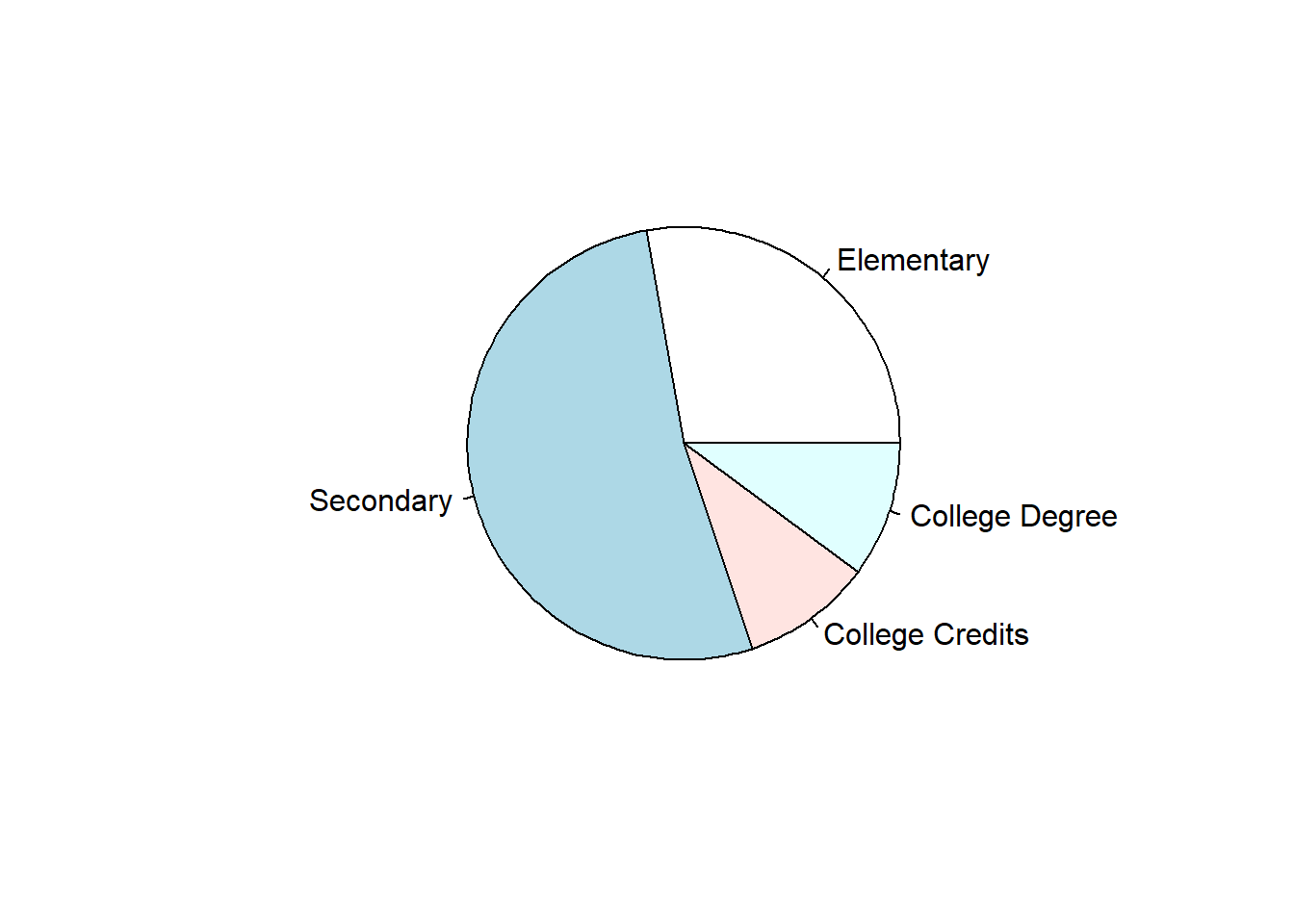

6.4 dotplot - for one numerical variable

library(mosaic)

# Notice that the "P" is captialized in dotPlot!
dotPlot(~width, data=KidsFeet, xlab = "width of foot (inches)")

dotPlot(~width, groups= sex, data=KidsFeet, pch=16,
        xlab = "width of foot (inches)")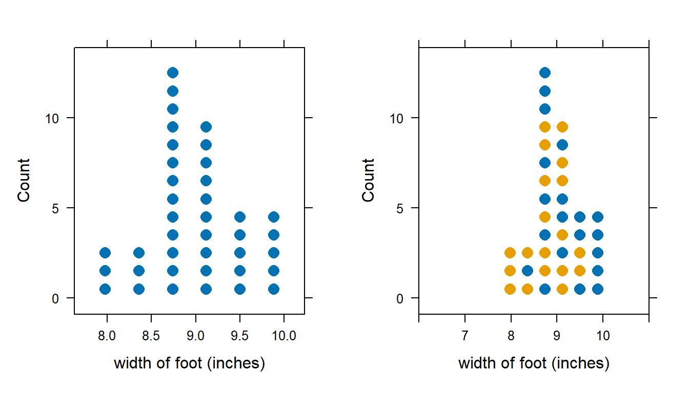

6.5 gf_dotPlot - for one numerical variable

library(ggformula)
gf_dotplot(~width, fill = ~sex, data=KidsFeet, binwidth = 0.1, 
        stackgroups = FALSE, 
        xlab = "width of foot (inches)")
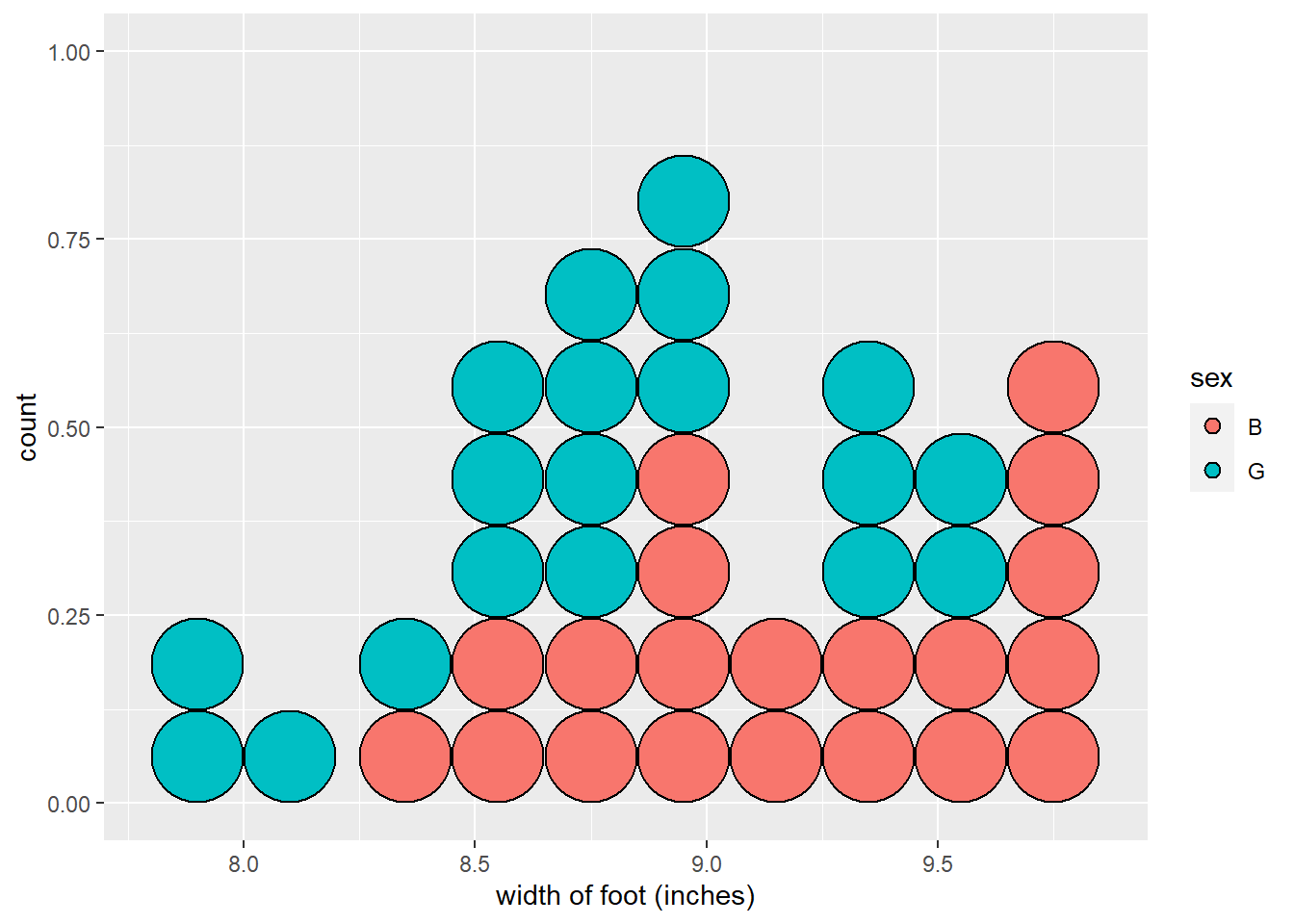
gf_dotplot(~width, fill = ~sex, data=KidsFeet, binwidth = 0.2, 
        stackgroups = TRUE, binpositions="all", 
        xlab = "width of foot (inches)")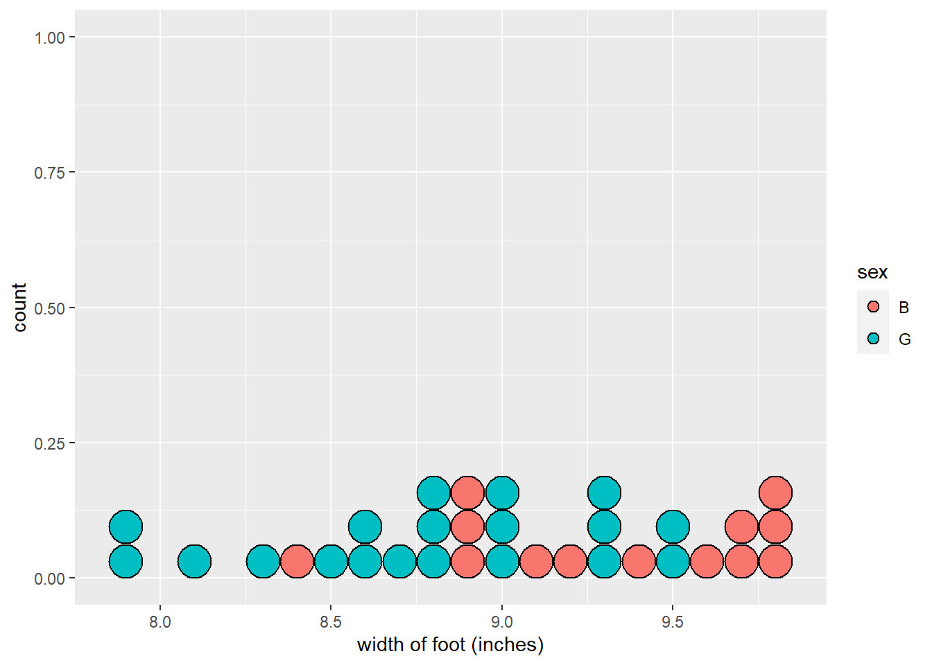

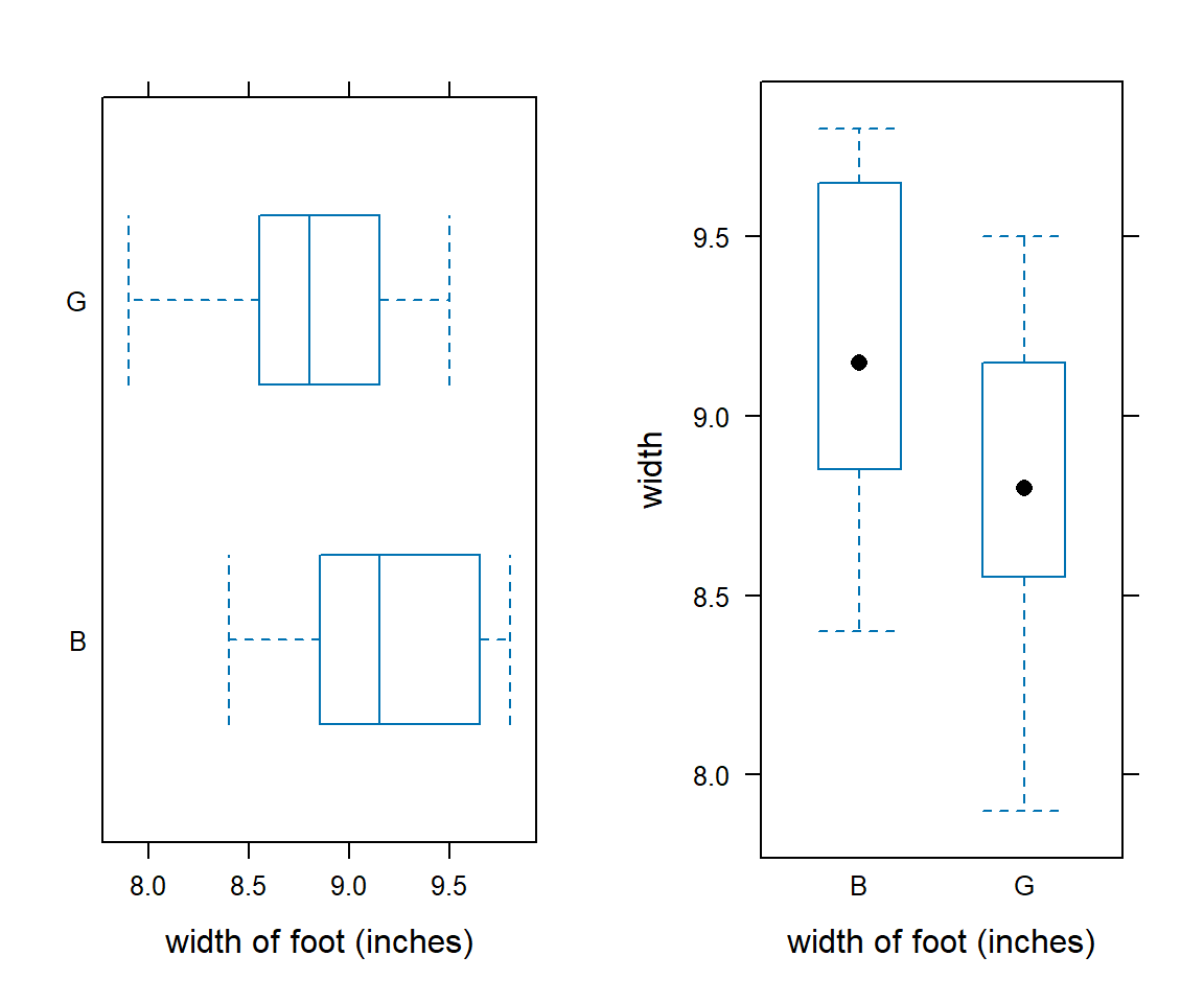
6.6 bwplot - for one numerical variable or one numerical/one categorical variable

library(mosaic)

bwplot(~width, data=KidsFeet, xlab = "width of foot (inches)")

bwplot(sex~width , data=KidsFeet, xlab = "width of foot (inches)")

bwplot(sex~width , data=KidsFeet, xlab = "width of foot (inches)", horizontal=TRUE, pch="|")

bwplot(width~sex , data=KidsFeet, xlab = "width of foot (inches)")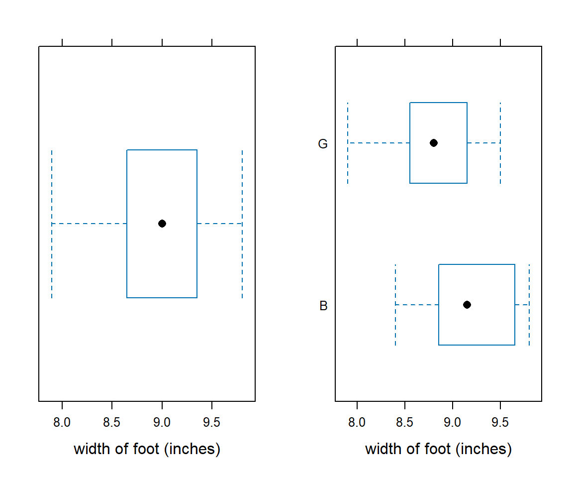

6.7 gf_histogram - for one numerical variable

library(ggformula)

gf_histogram(~width | sex, 
          binwidth = 0.25,
          xlim = c(7,11),
          ylab = "Percent of Students",              # y-axis label
          data=KidsFeet, xlab = "width of foot (inches)", 
          layout= c(2,1))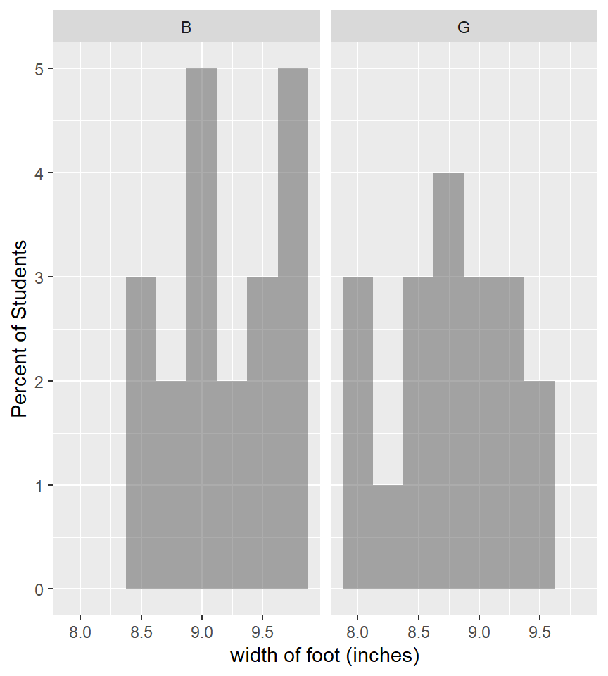

6.8 histogram - for one numerical variable

library(mosaic)

histogram(~width, data=KidsFeet, xlab = "width of foot (inches)")

histogram(~width | sex, data=KidsFeet, xlab = "width of foot (inches)", 
          layout= c(1,2))                       # layout using 1 column and 2 rows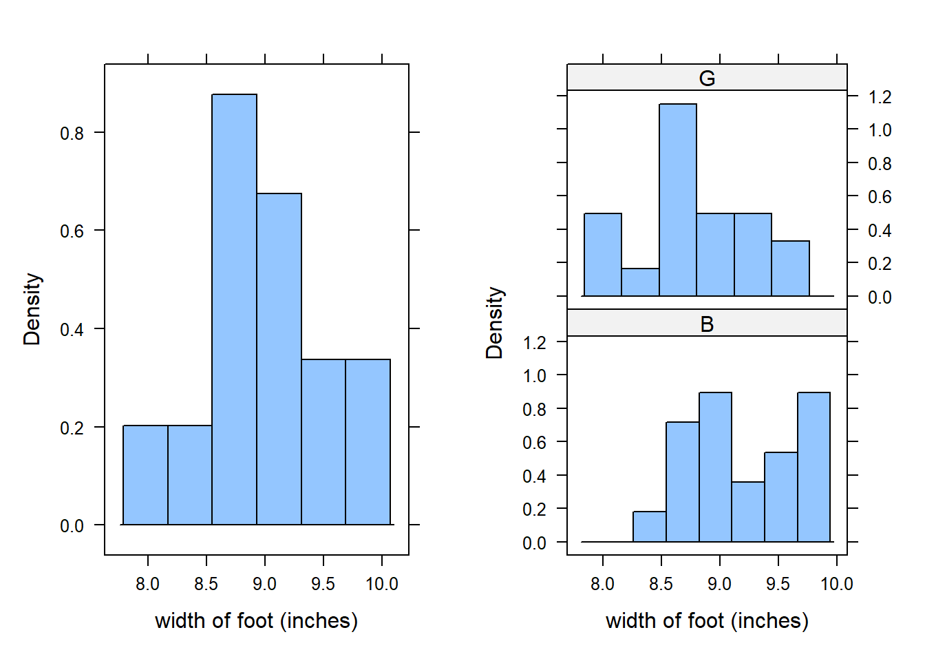

6.9 gf_boxplot - for one numerical variable

Notice that the ggformula function for a box-and-whisker plot is gf_boxplot (not gf_bwplot).

library(ggformula)

gf_boxplot(width~sex , data=KidsFeet)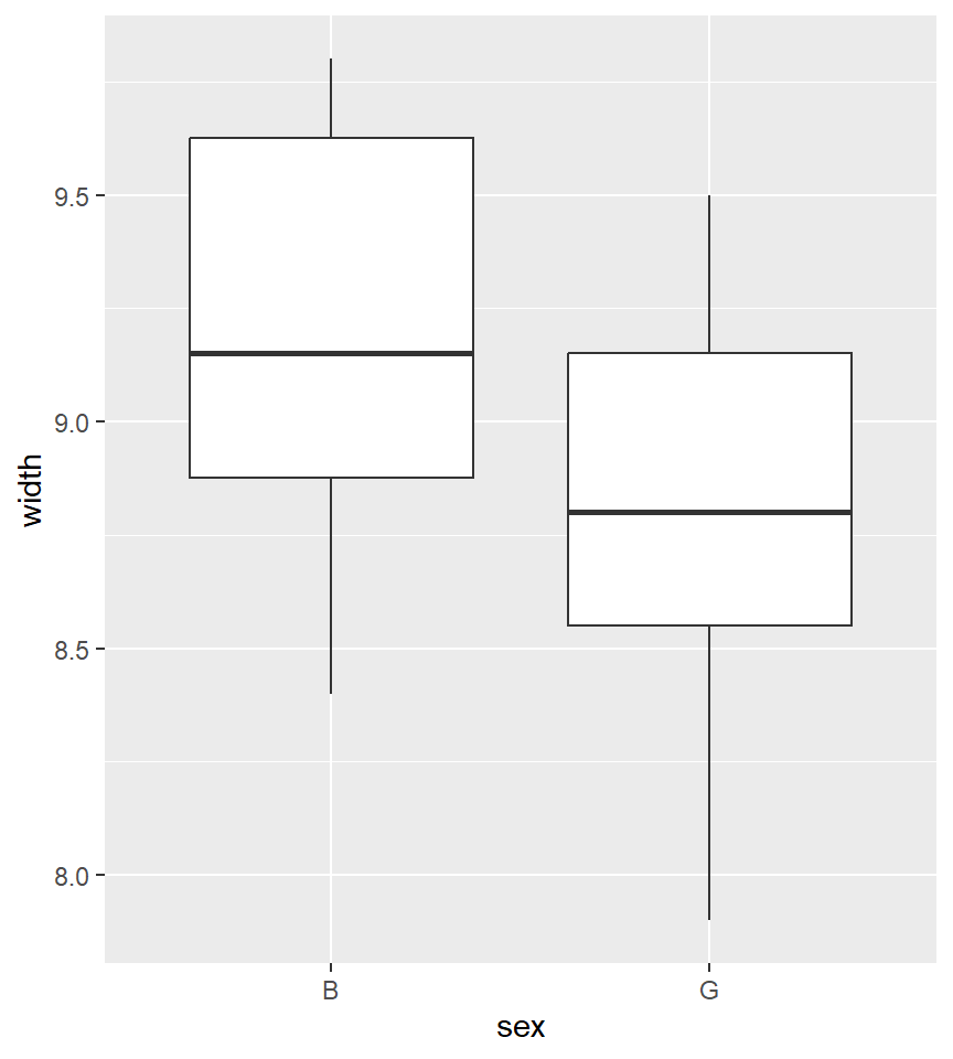

6.10 xyplot - for two numerical variables

An xyplot is also called a scatterplot.

library(mosaic)

xyplot(length~width, data=KidsFeet, xlab = "width of foot (inches)")

xyplot(length~width, groups=sex,  pch=16, cex = 1.4, 
       auto.key=list(space="right", title = "Gender", cex=.75), 
       data=KidsFeet, xlab = "width of foot (inches)")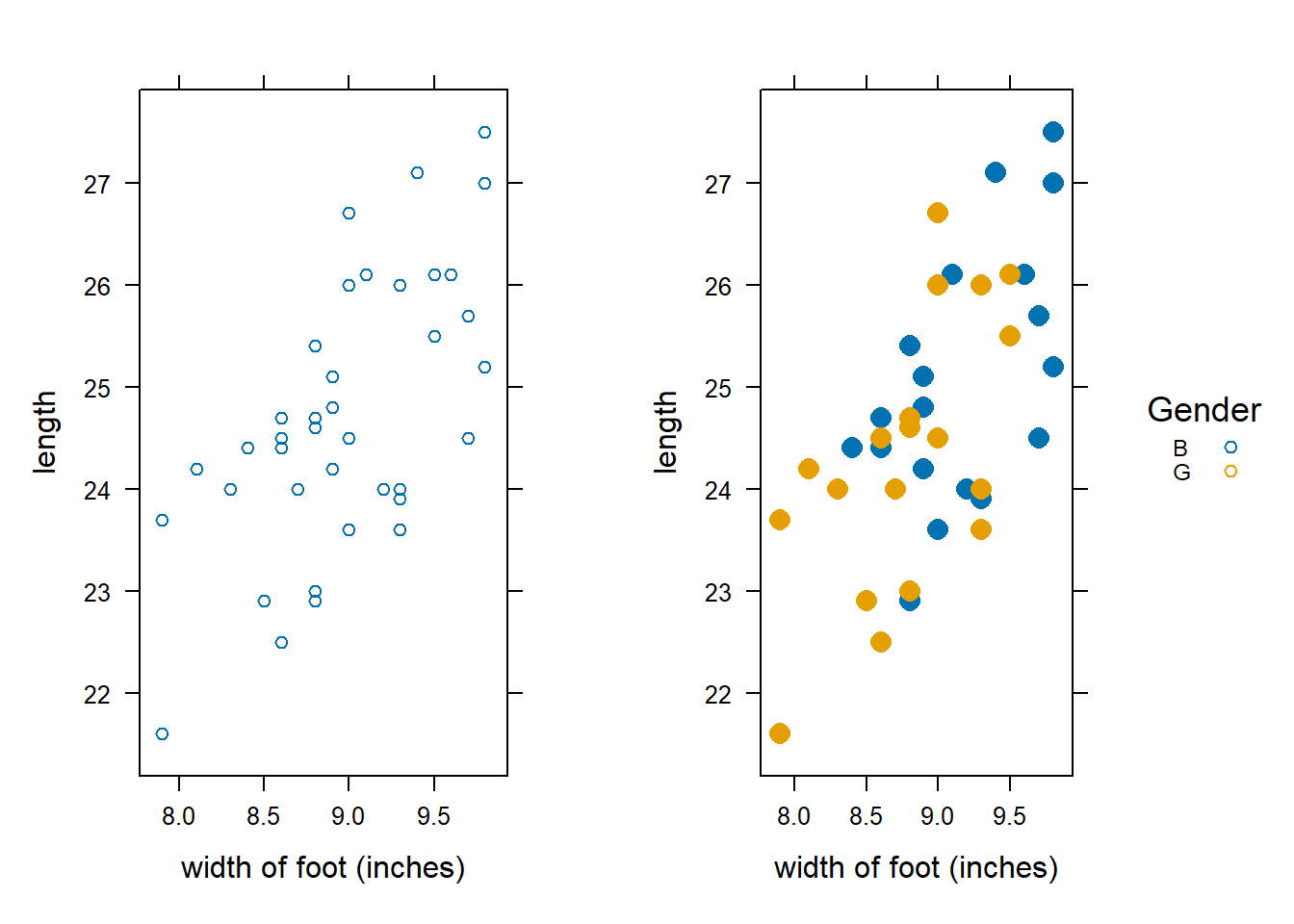

6.11 gf_xyplot - for two numerical variables

library(ggformula)

gf_point(length~width, data=KidsFeet,
         size = 3, color = ~ sex)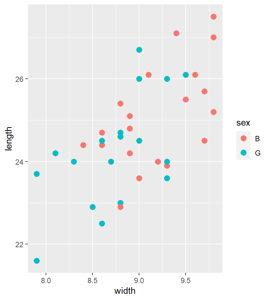

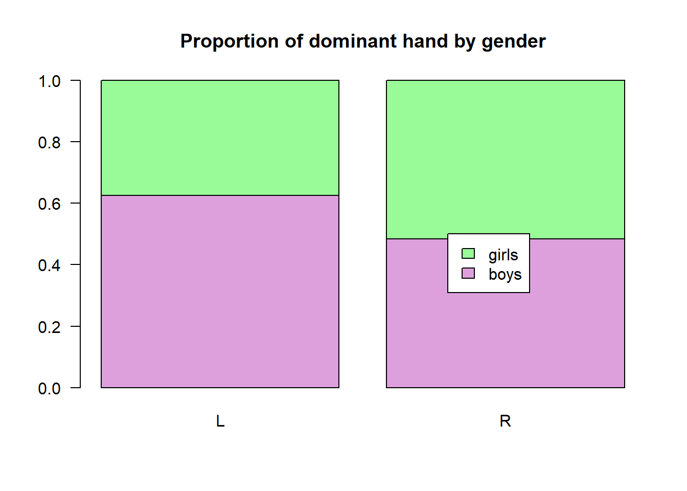
6.12 barplot - for comparing two proportions

tally(sex ~ domhand, data=KidsFeet)

##    domhand
## sex  L  R
##   B  5 15
##   G  3 16

barplot(prop.table(tally(sex ~ domhand, data=KidsFeet), margin = 2), 
        las = 1,   
        main = "Proportion of dominant hand by gender", 
        args.legend = list(x = 2, y = 0.5),
        # or args.legend = list(x = "bottomright")
        col = c("plum", "palegreen"),
        legend.text = c("boys", "girls"))