Chapter 1 Getting Started with RStudio
RStudio is an integrated development environment (IDE) for R that provides an alternative interface to R that has several advantages over other the default R interfaces:
RStudio runs on Mac, PC, and Linux machines and provides a simplified interface thatlooks and feels identical on all of them. The default interfaces for R are quite different on the various platforms. This can be distracting for the beginner.
RStudio can run in a web browser (using Rstudio.cloud) or on your personal computer.
RStudio provides support for reproducible research. RStudio makes it easy to include text, statistical analysis (R code and R output), and graphical displays all in the same document. The RMarkdown system provides a simple markup language and renders the results in HTML. The knitr/LATEX system allows users to combine R and LATEX in the same document. The reward for learning this more complicated system is much finer control over the output format. Depending on the level of the course, students can use either of these for homework and projects.
RStudio provides an integrated support for editing and executing R code and documents.
RStudio provides some useful functionality via a graphical user interface. RStudio is not a GUI for R, but it does provide a GUI that simplifies things like installing and updating packages; monitoring, saving and loading environments; importing and exporting data; browsing and exporting graphics; and browsing files and documentation.
1.1 Using RStudio Cloud
For very limited, occastional use of RStudio, you might use cloud-based version of RStudio, RStudio Cloud rather than a program installed on your computer. The “Cloud Free” level will allow you 15 hours per month of connect time.
You will want to create a new Project to store your files and data.
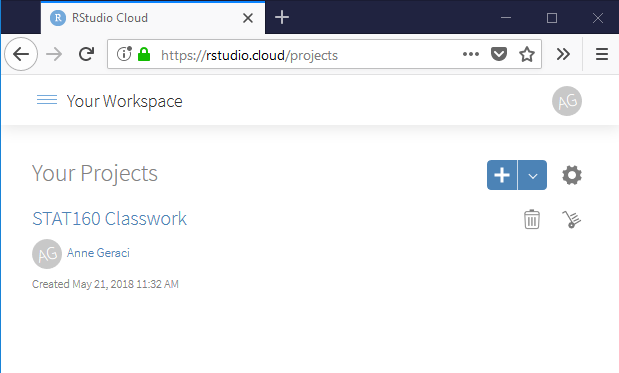
All your R programs will now be available from any computer using a web-browser.
1.2 Using RStudio on your personal computer
R and RStudio can be downloaded from the web as follows:
First download R from The R Project for Statistical Computing. Download and installation are pretty straightforward for Mac, PC, or Linux machines.
Next download {RStudio Desktop] (https://www.rstudio.com/products/rstudio/download/). Select the RStudio Desktop Free software appropriate for your Operating System. Install as instructed.
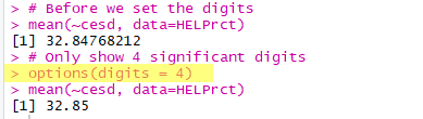
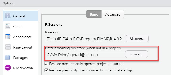
Finally, click on Tools/Global Options and set your working directory to the location on your computer where you will store your R scripts and data files.
1.3 RStudio Interface
Once you start RStudio, you will see the RStudio interface:
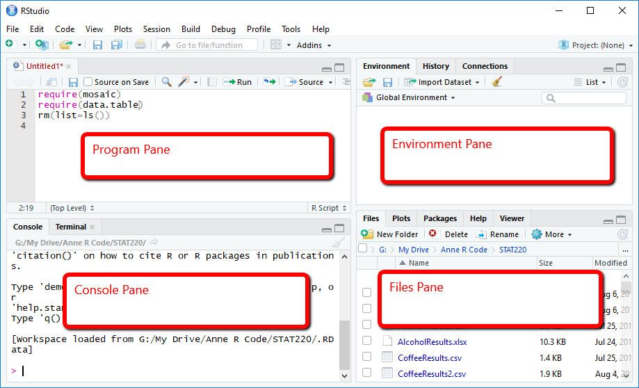
Notice that RStudio divides its world into four panels. Several of the panels are further subdivided into multiple tabs. Which tabs appear in which panels can be customized by the user. R can do much more than a simple calculator, and we will introduce additional features in due time. But performing simple calculations in R is a good way to begin learning the features of RStudio. Commands entered in the Console tab are immediately executed by R. A good way to familiarize yourself with the console is to do some simple calculator-like computations. Most of this will work just like you would expect from a typical calculator. Try typing the following command in the console panel.
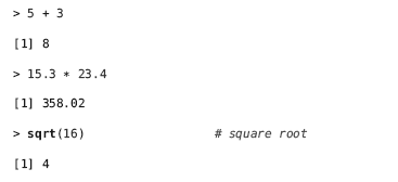
This last example demonstrates how functions are
called within R as well as the use of comments. Comments
are prefaced with the # character. Comments can
be very helpful when writing scripts with multiple commands
or to annotate example code for your students.
You can also save values to named variables for later reuse.
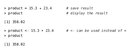
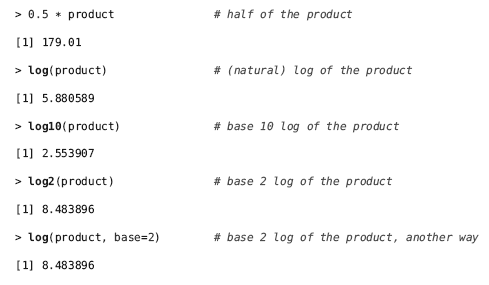
Once variables are defined, they can be referenced in other operations and functions
1.4 Working with R Script Files
Rather than typing R commands into the Console, we typically write short programs, known as “R scripts” that contain the R commands that we wish to execute. This allows for reproducibility because everytime you run your R script you’ll get the same result (assuming the input is the same). Or you could give your script to someone else and they’ll get the same result as well.
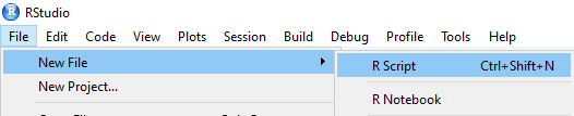
To To create a new R Script, select File, then New File, then R
Script from the RStudio menu. A file editor tab will open
in the Source panel. R code can be entered here, and buttons
and menu items are provided to run all the code
(called sourcing the file) or to run the code on a single
line or in a selected section of the file.
Use File, then Save to give your script a name and save it in your working directory.
Next, type the following commands into your R script:
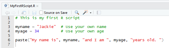
Note that any command that begins with a hash mark (#) is considered a comment and will not be evaluated by R.
You may now run each line of your script by clicking on the RUN button, or press the CTRL+ENTER keys simultaneously.
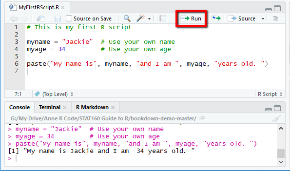
Notice that your results are now displayed in the Console window. Your R commands are shown with “>” and results are shown with “[1]”.
1.5 Using R Packages
Much of the functionality of R is provided through open-source “packages”, which are freely available for download from a central clearing website called CRAN (Comprehensive R Archive Network). There is a large community of R users who contribute various packages that do useful things like perform statistical procedures or produce custom output. Many packages also come with useful data files which can be used to learn how to use R commands.
Here are the packages that we will be using in this class:
- mosaic - Datasets and utilities from Project MOSAIC, used to teach math, statistics, computation and modeling.
- data.table - We will use the fread and fwrite functions for importing various types of data.
1.5.1 Installing a package
Before you start using an R package, you must first install it into your environment. The easiest way to do this is by clicking the Tools then Install Packages… menu option
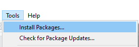
You only need to do this ONE time within your R environment.
1.5.2 Activating a package
To activate a package, use the require() or library() command. The two commands are identical except that require() will produce a more verbose output. If you are curious, you can type ‘require(mosaic)’ and ‘library(mosaic)’ to see the difference.
Here’s how to use the ‘library()’ command to activate the ‘mosaic’ package:
library(mosaic)
bwplot(wday~births, data=Births78)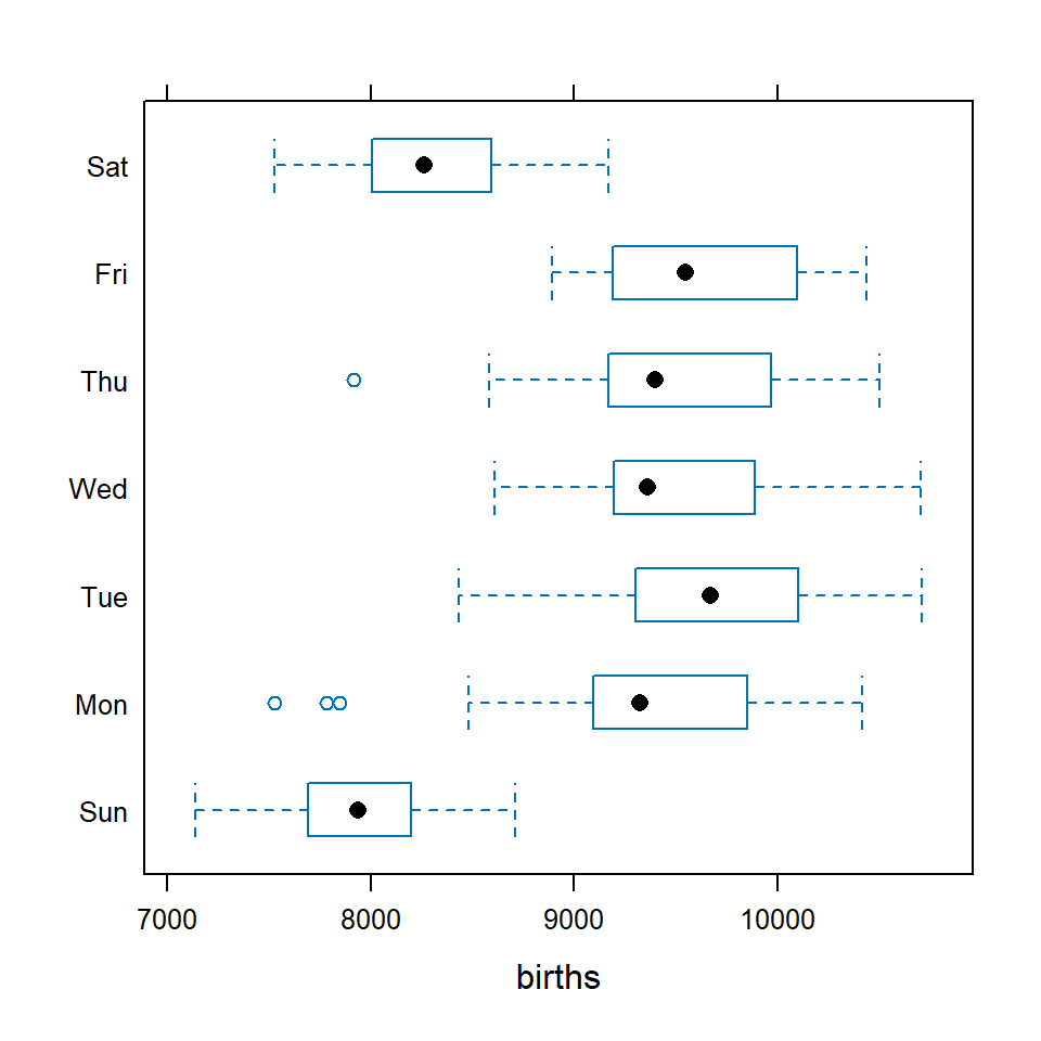
To learn more about a particular package, use the help (?) command. For example to find more information about the ‘mosaic’ package you could type ‘?mosaic’ in the Console window.
1.6 The Other Panels and Tabs
1.6.1 The History Tab
As commands are entered in the console, they appear in the History tab. These histories can be saved and loaded, there is a search feature to locate previous commands, and individual lines or sections can be transferred back to the console. Keeping the History tab open will allow you to go back and see the previous several commands. This can be especially useful when commands produce a fair amount of output and so scroll off the screen rapidly.
1.6.2 The Files Tab
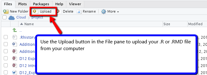
The Files tab provides a simple file manager. It can be navigated in familiar ways and used to open, move, rename, and delete files. In the browser version of RStudio, the Files tab also provides a file upload utility for moving files from the local machine to the server. In RMarkdown and knitr files one can also run the code in a particular chunk or in all of the chunks in a file. Each of these features makes it easy to try out code “live” while creating a document that keeps a record of the code.
In the reverse direction, code from the history can be copied either back into the console to run them again (perhaps after editing) or into one of the file editing tabs for inclusion in a file.
Use the Upload button in the Files tab to upload a script from your computer to RStudio Cloud.
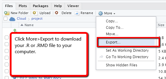
Use the More>Export button in the Files tab to downlad a script from RStudio Cloud.
 ### The Help Tab
The Help tab is where RStudio displays R help files. These
can be searched and navigated in the Help tab. You can
also open a help file using the ? operator in the console.
For example typing ‘?paste’ will provide the
help file for the paste function.
1.6.3 The Environment Tab
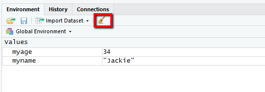
The Environment tab shows the variables that you’ve created and objects available to the
console. These are subdivided into data, values (nondataframe,
non-function objects) and functions. The
broom icon can be used to remove all objects from the environment,
and it is good to do this from time to time. The ‘rm(list=ls())’ command will do the same thing.
1.6.4 The Plots Tab
Plots created in the console are displayed in the Plots tab. For example, the following commands display the number of births in the United States for each day in 1978.
# activating the mosaic package will make lattice graphics available to the session
# as well as the Births78 dataset
library(mosaic)
xyplot(births ~ day_of_year, data=Births78)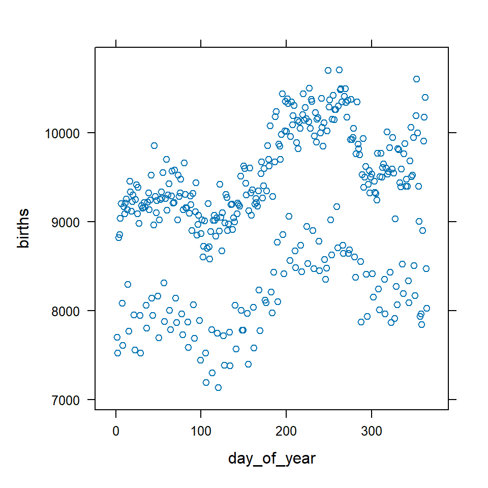
From the Plots tab, you can navigate to previous plots and also export plots in various formats after interactively resizing them.
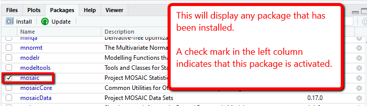 The Packages tab displays which package are installed and/or loaded into your environment.
It will also allow you to search for packages that
have been updated since you installed them.
The Packages tab displays which package are installed and/or loaded into your environment.
It will also allow you to search for packages that
have been updated since you installed them.1.7 Important things to know about R
1.7.1 R is case-sensitive
If you mis-capitalize something in R it won’t do what you want. Pay careful attention to the spelling and capitalization of variables and datasets.
A variable named ‘Mydata’ is not the same as one named ‘mydata’.
1.7.2 Special characters used by R:
- ~ (tilde) - found in the upper left corner of the keyboard (must use SHIFT). This is used in many commands to separate parameters, as in “time ~ group”.
- ` (back-tic) - found in the upper left corner of the keyboard. This is used as a delimeter for strings, as in
this is a string - ' (single quote) - found on the right side of the keyboard next to ENTER. This is used for …..
1.7.3 Common Errors from R:
- If you see a + prompt in the Console, it means R is waiting for more input. Often this means that you have forgotten a closing parenthesis or made dome other syntax error.
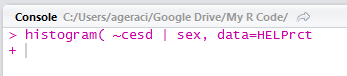
How to fix it: Press ESC key to return to the > prompt and start the command fresh.
Error in xxxxxxxxx : object ‘xxxx’ not found
R was not expecting to find “xxxx” where it did. You probably either misspelled something, forgot a comma, or put the arguments in the incorrect order.
What happens if you use a function before loading the library ….
1.8 Useful options and commands
1.8.1 How to clear your environment
The following command should be used at the top of every R script you write. It will clear out any environment variables that you may have stored in a prior R session.

In order for your R code to be reproducible you must start with a blank slate (empty environment) every time you run the code.