Chapter 2 Algorithms
To make R do anything at all, you write an R script. In your R script, you tell the computer, step by step, exactly what you want it to do, in the proper order. R then executes each line of your script, following each step according to how you have designe the script.
When you are telling the computer what to do, you also get to choose how it’s going to be done. That’s where computer algorithms come in. An algorithm is the basic technique used to get the job done. For example, let’s say you have a friend arriving at the airport and she needs to get from the airport to your house. She might use the following algorithm:
- Catch bus number 70 outside the baggage claim area
- Transfer to bus 14 on Main St.
- Get off at Elm St.
- Walk two blocks north to my house.
You will note that the algorighm is written in the order in which it is to be executed. It wouldn’t make sense to perform Step 4 (Walk two blocks north) until after the other three steps have been computed.
An R script is also written as an algorithm.
2.1 Example 1: Color Names
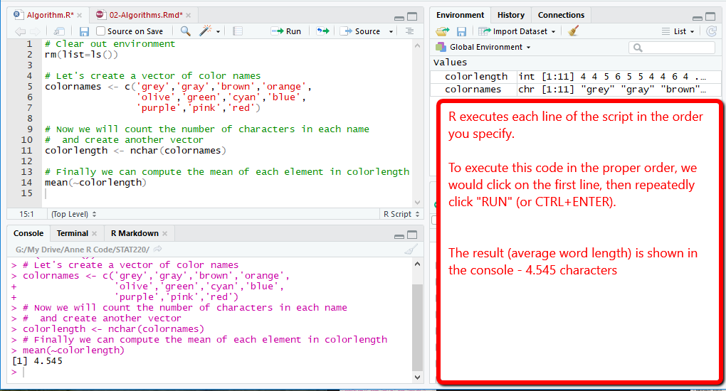
Let’s say we have a bunch of words - say, the names of colors. We want to compute the average number of characters in these words. If we were going to do this by hand, we would use the following algorithm:
- Create a list of the words
- Count the number of characters in each word
- Compute the average from Step 2.
Here’s what this algorithm would look like in R:
2.2 Example 2: Flipping a Coin
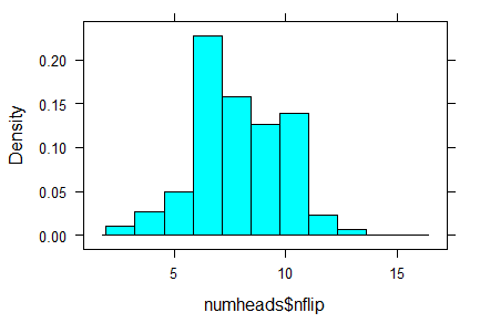
Here’s another example. Let’s say we want to simulate lots and lots (like, 1000) of trials of flipping 16 pennies. We want to investigate the distribution of the number of heads we get when we flip that many pennies.
That would take a long time to do by hand, but with R we can simulate flipping a coin with the nflip() function.
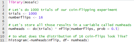
We flip the 16 coins 1000 times and count the number of heads on each trial. Since it is a fair coin (we used p = 0.5), we expect to get a distribution centered around 8. The following output confirms this result.
2.3 Example 3: A typical Data Science algorithm
When we are doing data science, we typically will us an algorithm that looks something like this:
2.3.0.1 Step 1: Read in the Data
# Read the data from the web somewhere
df <- read.csv("http://citadel.sjfc.edu/faculty/ageraci/data/GummyBears.csv")
str(df)
## 'data.frame': 264 obs. of 4 variables:
## $ Group : chr "A" "A" "A" "A" ...
## $ Blocks : int 1 1 1 1 1 1 1 1 5 5 ...
## $ Ramp : chr "top" "top" "top" "top" ...
## $ Distance: num 40 56 48 54 59 49 53 58 70 76 ...2.3.0.2 Step 2: Select the variables of interest
"Gummy Bears Data"## [1] "Gummy Bears Data"df2 <- select(df, Group, Distance)
str(df2)## 'data.frame': 264 obs. of 2 variables:
## $ Group : chr "A" "A" "A" "A" ...
## $ Distance: num 40 56 48 54 59 49 53 58 70 76 ...2.3.0.3 Step 3 Filter your data to the desired subset of rows
"Gummy Bears Data"## [1] "Gummy Bears Data"df3 <- filter(df2, Group %in% c("A","B"))
str(df3)## 'data.frame': 48 obs. of 2 variables:
## $ Group : chr "A" "A" "A" "A" ...
## $ Distance: num 40 56 48 54 59 49 53 58 70 76 ...2.3.0.4 Step 4 Create computed variables with mutate
If you need to create any computed variables in your data frame, use the mutate operation. Let’s say we want to create a variable called Distance.HighLow, which will be “High” if the Distance is above the average for the group and otherwise “Low”.
df4 <- mutate(df3, Distance.HighLow =
                ifelse(Distance < mean(~Distance, data=df3, na.rm=T), "Low", "High"))
str(df4)
## 'data.frame': 48 obs. of 3 variables:
## $ Group : chr "A" "A" "A" "A" ...
## $ Distance : num 40 56 48 54 59 49 53 58 70 76 ...
## $ Distance.HighLow: chr "Low" "Low" "Low" "Low" ...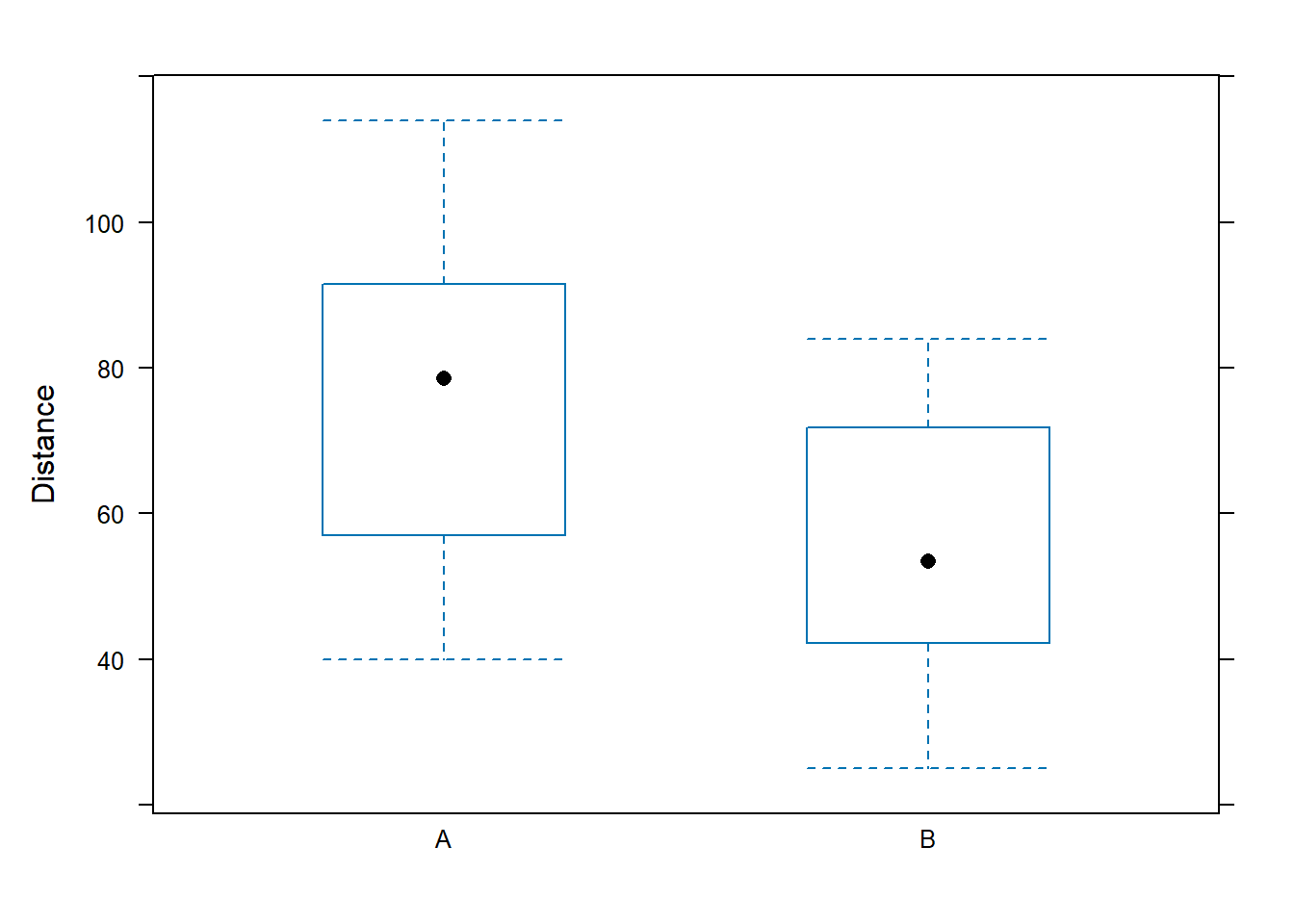
2.4 Example 3: A typical Data Science algorithm - Using Pipes
We can also chain together the above statements in a single chunk of code, as follows:
# read the data ... and then select .... and then filter
df.gb <- fread("http://citadel.sjfc.edu/faculty/ageraci/data/GummyBears.csv") %>%
  select( Group, Distance) %>%
  filter( Group %in% c("A", "B")) %>%
  mutate( Distance.HighLow =
                ifelse(Distance < mean(~Distance, data=df3, na.rm=T), "Low", "High"))
str(df.gb)
## Classes 'data.table' and 'data.frame': 48 obs. of 3 variables:
## $ Group : chr "A" "A" "A" "A" ...
## $ Distance : num 40 56 48 54 59 49 53 58 70 76 ...
## $ Distance.HighLow: chr "Low" "Low" "Low" "Low" ...
## - attr(*, ".internal.selfref")=<externalptr>favstats(~Distance | Group, data=df.gb)## Group min Q1 median Q3 max mean sd n missing
## 1 A 40 57.500 78.5 91.250 114 74.33333 19.14627 24 0
## 2 B 25 42.375 53.5 70.875 84 55.43750 16.91880 24 02.5 Example 4 - Saratoga Houses
Here’s another example using the data file SaratogaHouses, which is found within the MosaicData package.
str(SaratogaHouses)## 'data.frame': 1728 obs. of 16 variables:
## $ price : int 132500 181115 109000 155000 86060 120000 153000 170000 90000 122900 ...
## $ lotSize : num 0.09 0.92 0.19 0.41 0.11 0.68 0.4 1.21 0.83 1.94 ...
## $ age : int 42 0 133 13 0 31 33 23 36 4 ...
## $ landValue : int 50000 22300 7300 18700 15000 14000 23300 14600 22200 21200 ...
## $ livingArea : int 906 1953 1944 1944 840 1152 2752 1662 1632 1416 ...
## $ pctCollege : int 35 51 51 51 51 22 51 35 51 44 ...
## $ bedrooms : int 2 3 4 3 2 4 4 4 3 3 ...
## $ fireplaces : int 1 0 1 1 0 1 1 1 0 0 ...
## $ bathrooms : num 1 2.5 1 1.5 1 1 1.5 1.5 1.5 1.5 ...
## $ rooms : int 5 6 8 5 3 8 8 9 8 6 ...
## $ heating : Factor w/ 3 levels "hot air","hot water/steam",..: 3 2 2 1 1 1 2 1 3 1 ...
## $ fuel : Factor w/ 3 levels "gas","electric",..: 2 1 1 1 1 1 3 3 2 1 ...
## $ sewer : Factor w/ 3 levels "septic","public/commercial",..: 1 1 2 1 2 1 1 1 1 3 ...
## $ waterfront : Factor w/ 2 levels "Yes","No": 2 2 2 2 2 2 2 2 2 2 ...
## $ newConstruction: Factor w/ 2 levels "Yes","No": 2 2 2 2 1 2 2 2 2 2 ...
## $ centralAir : Factor w/ 2 levels "Yes","No": 2 2 2 2 1 2 2 2 2 2 ...favstats(~price | fuel,data=SaratogaHouses)## fuel min Q1 median Q3 max mean sd n missing
## 1 gas 5000 159000 206500 276000 775000 228535.1 102186.88 1197 0
## 2 electric 10300 122750 149300 187750 475000 164937.6 68084.35 315 0
## 3 oil 20000 135000 167500 225000 620000 188734.4 87593.64 216 0# Look at Price, bedrooms, sewer, and fireplaces for only 4 bedroom houses
df.houses <- SaratogaHouses %>%
select(price, bedrooms, sewer, fuel, fireplaces) %>%
filter(bedrooms == 4) %>%
mutate(fp.YesNo = ifelse(fireplaces == 0, "No", "Yes") ,
fuel.2state = ifelse(fuel %in% c("gas","oil"), "Fossil Fuel", "Electric"))
str(df.houses)## 'data.frame': 487 obs. of 7 variables:
## $ price : int 109000 120000 153000 170000 253750 248800 145000 457000 179900 169900 ...
## $ bedrooms : int 4 4 4 4 4 4 4 4 4 4 ...
## $ sewer : Factor w/ 3 levels "septic","public/commercial",..: 2 1 1 1 3 1 1 2 1 1 ...
## $ fuel : Factor w/ 3 levels "gas","electric",..: 1 1 3 3 1 3 3 3 1 1 ...
## $ fireplaces : int 1 1 1 1 1 0 0 1 1 1 ...
## $ fp.YesNo : chr "Yes" "Yes" "Yes" "Yes" ...
## $ fuel.2state: chr "Fossil Fuel" "Fossil Fuel" "Fossil Fuel" "Fossil Fuel" ...favstats(~price | fuel.2state, data=df.houses)## fuel.2state min Q1 median Q3 max mean sd n
## 1 Electric 65000 188000 217000.0 278500.0 380000 229979.3 80300.05 29
## 2 Fossil Fuel 78500 197400 253204.5 318827.5 725000 267803.0 97291.65 458
## missing
## 1 0
## 2 0