Chapter 3 All about Data in R
3.1 Using data that is built into R
Some times we can just use data that is built into an R package. This is mostly for instructional purposes since this data has already been analyzed. For example, the mtcars data set has a number of
str(mtcars)## 'data.frame': 32 obs. of 11 variables:
## $ mpg : num 21 21 22.8 21.4 18.7 18.1 14.3 24.4 22.8 19.2 ...
## $ cyl : num 6 6 4 6 8 6 8 4 4 6 ...
## $ disp: num 160 160 108 258 360 ...
## $ hp : num 110 110 93 110 175 105 245 62 95 123 ...
## $ drat: num 3.9 3.9 3.85 3.08 3.15 2.76 3.21 3.69 3.92 3.92 ...
## $ wt : num 2.62 2.88 2.32 3.21 3.44 ...
## $ qsec: num 16.5 17 18.6 19.4 17 ...
## $ vs : num 0 0 1 1 0 1 0 1 1 1 ...
## $ am : num 1 1 1 0 0 0 0 0 0 0 ...
## $ gear: num 4 4 4 3 3 3 3 4 4 4 ...
## $ carb: num 4 4 1 1 2 1 4 2 2 4 ...head(mtcars)## mpg cyl disp hp drat wt qsec vs am gear carb
## Mazda RX4 21.0 6 160 110 3.90 2.620 16.46 0 1 4 4
## Mazda RX4 Wag 21.0 6 160 110 3.90 2.875 17.02 0 1 4 4
## Datsun 710 22.8 4 108 93 3.85 2.320 18.61 1 1 4 1
## Hornet 4 Drive 21.4 6 258 110 3.08 3.215 19.44 1 0 3 1
## Hornet Sportabout 18.7 8 360 175 3.15 3.440 17.02 0 0 3 2
## Valiant 18.1 6 225 105 2.76 3.460 20.22 1 0 3 13.2 Importing Data from .CSV file using read.csv or read.delim
- If your data is in your working directory (the same directory where your program is):
df <- read.csv("GummyBears.csv")

str(df)
## 'data.frame': 96 obs. of 4 variables:
## $ Group : chr "A" "A" "A" "A" ...
## $ Blocks : int 1 1 1 1 1 1 1 1 1 1 ...
## $ Ramp : int 1 1 1 1 1 1 1 1 1 1 ...
## $ Distance: num 65 78 45.5 50 46 23.5 13 35.5 83 74 ...- If your data is on the web somewhere:
df <- read.csv("http://citadel.sjfc.edu/faculty/ageraci/data/GummyBears.csv")

str(df)
## 'data.frame': 264 obs. of 4 variables:
## $ Group : chr "A" "A" "A" "A" ...
## $ Blocks : int 1 1 1 1 1 1 1 1 5 5 ...
## $ Ramp : chr "top" "top" "top" "top" ...
## $ Distance: num 40 56 48 54 59 49 53 58 70 76 ...3.3 Importing Data from .CSV file using fread
- If your data is in your working directory (the same directory where your program is):
library(data.table)

# This command creates a dataframe called “df”
df <- fread("GummyBears.csv")

str(df)
## Classes 'data.table' and 'data.frame': 96 obs. of 4 variables:
## $ Group : chr "A" "A" "A" "A" ...
## $ Blocks : int 1 1 1 1 1 1 1 1 1 1 ...
## $ Ramp : int 1 1 1 1 1 1 1 1 1 1 ...
## $ Distance: num 65 78 45.5 50 46 23.5 13 35.5 83 74 ...
## - attr(*, ".internal.selfref")=<externalptr>- If your data is on the web somewhere:
library(data.table)

df <- fread("http://citadel.sjfc.edu/faculty/ageraci/data/GummyBears.csv")

str(df)
## Classes 'data.table' and 'data.frame': 264 obs. of 4 variables:
## $ Group : chr "A" "A" "A" "A" ...
## $ Blocks : int 1 1 1 1 1 1 1 1 5 5 ...
## $ Ramp : chr "top" "top" "top" "top" ...
## $ Distance: num 40 56 48 54 59 49 53 58 70 76 ...
## - attr(*, ".internal.selfref")=<externalptr>3.4 Importing Data from a TXT file
What if your data is in TXT format?
df <- read.delim("http://citadel.sjfc.edu/faculty/ageraci/data/tuna.txt")

str(df)
## 'data.frame': 274 obs. of 2 variables:
## $ Tuna : chr "albacore " "albacore " "albacore " "albacore " ...
## $ Mercury: num 0 0.41 0.82 0.32 0.036 0.28 0.29 0.34 0.36 0.42 ...3.5 Importing Data from Excel (.xlsx) file
library(readxl)

df <- read_xls("SalaryData.xls")

str(df)
## tibble [497 × 6] (S3: tbl_df/tbl/data.frame)
## $ Employee : num [1:497] 1 2 3 4 5 6 7 8 9 10 ...
## $ Gender : num [1:497] 1 0 0 1 0 0 0 1 1 0 ...
## $ Education: num [1:497] 0 3 3 3 3 4 3 2 0 4 ...
## $ Age : num [1:497] 24 39 27 43 36 40 38 30 31 52 ...
## $ YrsExp : num [1:497] 1 2 2 8 2 8 3 1 6 6 ...
## $ Salary : num [1:497] 40.8 57 52.6 52 49.2 61.1 52.3 42.9 34.9 55 ...3.6 Creating Raw Data from Summary Data
Let’s say we only have summary level data, as in this table of counts:
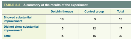
In order to create a data table with individual rows for each subject, we use the data.table command.
library(data.table)
df <- data.table(Group = c(rep("dolphin", 15),
                           rep("control",15)),
                 Improve = c(rep("yes",10), rep("no",5),
                             rep("yes",3), rep("no", 12)))
3.7 Creating output from R
Occasionally, you may need to save your R data to an external file so that you can share it with someone else. In this case, we will use the fwrite function, which is a good complement to fread.
library(data.table)
fwrite(mtcars,"mtcars.csv")
3.8 Data frames
Data sets in R are usually stored in objects that we call data frames. A dataframe is a rectangular arrangement of data with rows corresponding to observational units and columns corresponding to variables.
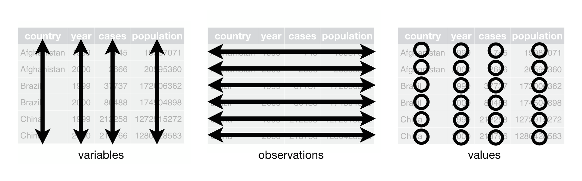
For example, the mtcars data frame is an arrangment of data where each row pertains to one model of car, and the columns contain measurements or other characteristics about that model.
head(mtcars)## mpg cyl disp hp drat wt qsec vs am gear carb
## Mazda RX4 21.0 6 160 110 3.90 2.620 16.46 0 1 4 4
## Mazda RX4 Wag 21.0 6 160 110 3.90 2.875 17.02 0 1 4 4
## Datsun 710 22.8 4 108 93 3.85 2.320 18.61 1 1 4 1
## Hornet 4 Drive 21.4 6 258 110 3.08 3.215 19.44 1 0 3 1
## Hornet Sportabout 18.7 8 360 175 3.15 3.440 17.02 0 0 3 2
## Valiant 18.1 6 225 105 2.76 3.460 20.22 1 0 3 1