Chapter 8 Modeling

8.1 Correlation

To compute the correlation between two variables, we use the ‘cor()’ function:

df <- fread("http://citadel.sjfc.edu/faculty/ageraci/data/ExamTimesScores.txt")
str(df)

## Classes 'data.table' and 'data.frame':   30 obs. of  2 variables:
##  $ time : int  30 41 41 43 47 48 51 54 54 56 ...
##  $ score: int  100 84 94 90 88 99 85 84 94 100 ...
##  - attr(*, ".internal.selfref")=<externalptr>

(correlation <- cor(score ~ time, data=df,use = "complete.obs"))

## [1] -0.125

8.2 Scatterplot

xyplot(score ~ time, data=df, 
       main = "Exam time vs. Score", 
       xlab = "Time (in minutes)", 
       ylab = "Score on Exam", 
       type = c("p", "r"), 
       pch = 16, cex = 1.2)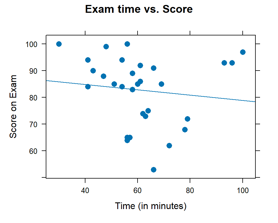

8.3 Linear Regression:

(mod <- lm(score ~ time, data=df))

## 
## Call:
## lm(formula = score ~ time, data = df)
## 
## Coefficients:
## (Intercept)         time  
##     88.8751      -0.0996

8.4 Residual Diagnostic Graphs

xyplot(resid(mod) ~ predict(mod), xlab="Fitted Values", 
       ylab="Residual Values", pch = 16, cex = 1.5, 
       main = "Residual vs. Fitted Diagnostic Graph",
       data=df)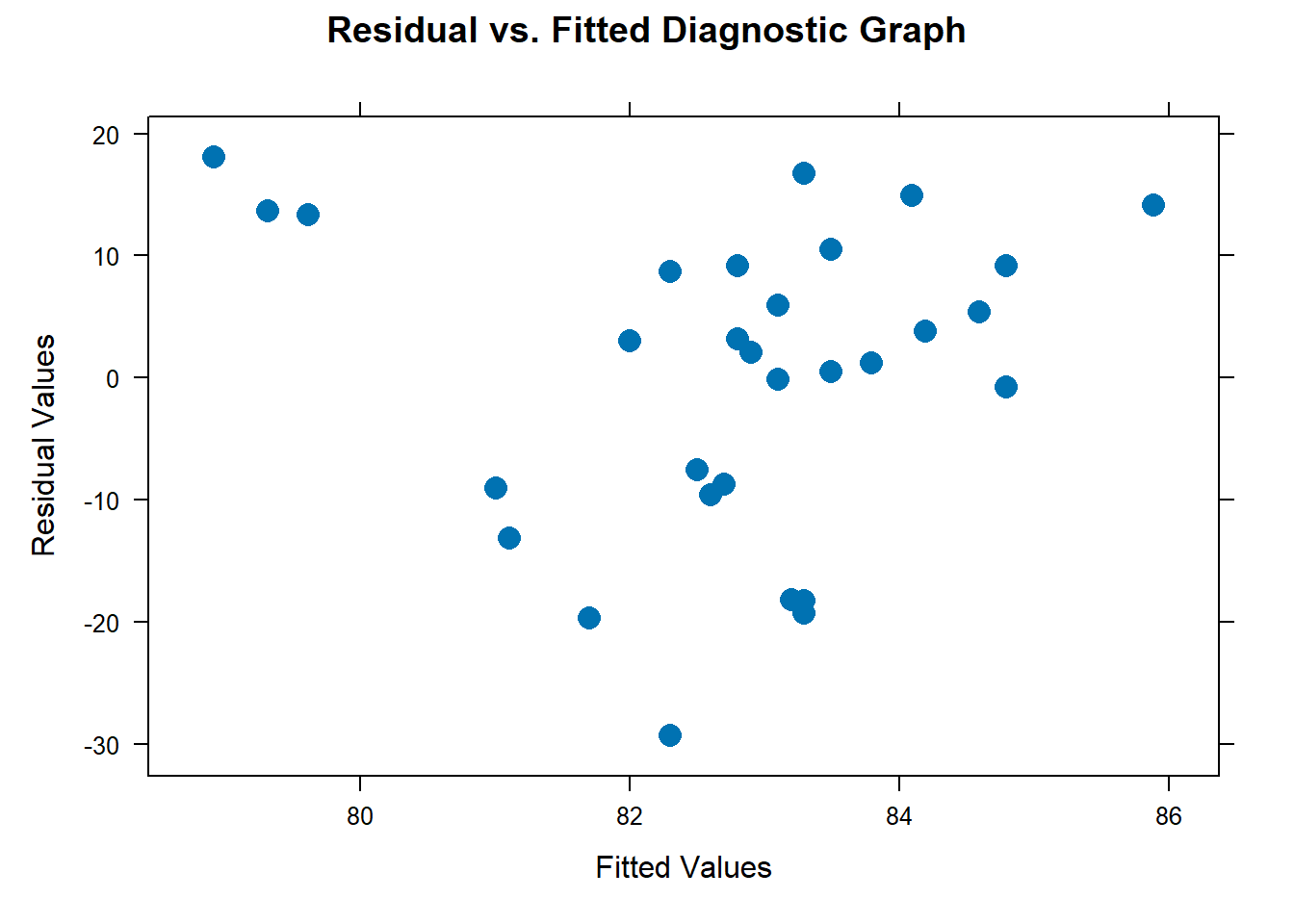

xyplot(fitted.values ~ model$time, xlab="Observed Values", 
       ylab="Fitted Values", 
       pch = 16, cex = 1.5,
       main = "Fitted vs. Actual Diagnostic Graph", 
       type = c("p", "r"), data=mod)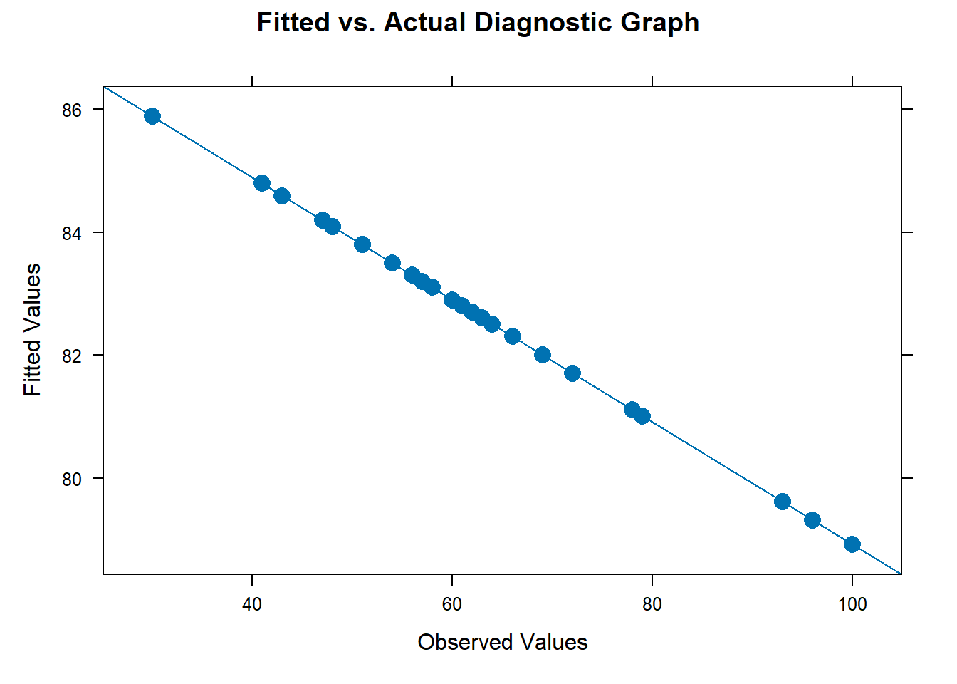

8.5 Making predictions

"Score Prediction for time = 45 minutes"

## [1] "Score Prediction for time = 45 minutes"

predict(mod, data.frame(time = 45))

##      1 
## 84.393

"Score Prediction for time = 70 minutes"

## [1] "Score Prediction for time = 70 minutes"

predict(mod, data.frame(time = 70))

##      1 
## 81.904