Chapter 4 All about functions
4.1 Functions
One of the great strengths of R is the ability to use pre-written functions. There are functions for all sorts of things, from creating statistical results to parsing huge datafiles from the internet.
Functions in R are written using the following syntax:
functionname( argument1, argument2, ... )The arguments are always surrounded by (round) parentheses and separated by commas. some functions (like ‘data()’) have no required arguments, but you still need the parentheses.
For example, here are some R functions that compute various mathematical quantities. Type them to see if you can guess what they do.
sqrt(144) This is a function that computes the square root of whatever is inside the parenthases. The value 144 is passed as an argument to the function sqrt.
mean(c(4,10,5,8,12))The mean function, used to compute the mathematical average, takes an argument that contains the numbers that are to be included in computing the average. In this case, we have created a vector (that’s a term you’ll learn about in the DataCamp Intro to R course) with five elements. When we pass that vector to the mean function as an argument, the function returns the mathematical average.
# Create a vector with five elements
c(4,10,5,8,12)
## [1] 4 10 5 8 12To learn about any function, type a question mark (?) followed by the function into the R console. Try this one:
?mean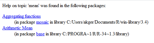
In this case, R tells you that the function mean was found in package mosaic and in the base (built-in) R libraries. In general, if you have a choice like this, pick the function in package mosaic.
4.2 Functions - mosaic-style
Most of what we will do in this class will make use of functions according to the following R mosaic-style template:
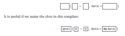
However, there are some variations on this template: As you can see, the mosaic-style formula template requires the FIRST argument to be a formula.
# Simpler version
goal( ~ x, data = mydata )

# Fancier version:
goal( y ~ x | z , data = mydata )
To use the template, you just need to know what to use for x, y, z, and mydata. This can be determined by asking yourself two questions:
What do you want R to do? This determines what function to use (goal).
What must R know to do that? This determines the inputs to the function. For example, we need to identify which data frame and which variable(s).
Further, if you begin type a function and hit the TAB key, will show you a list of possible ways to complete the command. If you hit TAB after the opening parenthesis of a function, it will show you the list of arguments it expects. The up and down arrows can be used to retrieve past commands.
For example, if your goal is to compute a mean (question 1) and your data resides in a data frame called KidsFeet stored in a variable called width (question 2), then you would code the following:
library(mosaicData)
mean(~width,  data=KidsFeet, na.rm=T)
## [1] 8.992308Note that the “squiggle” (~) character, also called a tilde, is required to tell R how to parse the formla.
Here’s an example of a function, tally(), that can accept variables on both sides of the “squiggle”:
tally(domhand ~ sex, data=KidsFeet)## sex
## domhand B G
## L 5 3
## R 15 164.3 Functions - Data frames
Now that we’ve explained a few basics for using R, let’s look at some functions that might help us do something useful.
We’ll be using one of the built-in datasets that is provided with base R, called iris. This dataset contains 50 samnples from each of three species of the iris plants. Four features were measured from each sample: the length and width of the sepals and petals, in centimeters.
We can view the variables, known as the “structure” of the dataset, using the str() command.
str(iris)## 'data.frame': 150 obs. of 5 variables:
## $ Sepal.Length: num 5.1 4.9 4.7 4.6 5 5.4 4.6 5 4.4 4.9 ...
## $ Sepal.Width : num 3.5 3 3.2 3.1 3.6 3.9 3.4 3.4 2.9 3.1 ...
## $ Petal.Length: num 1.4 1.4 1.3 1.5 1.4 1.7 1.4 1.5 1.4 1.5 ...
## $ Petal.Width : num 0.2 0.2 0.2 0.2 0.2 0.4 0.3 0.2 0.2 0.1 ...
## $ Species : Factor w/ 3 levels "setosa","versicolor",..: 1 1 1 1 1 1 1 1 1 1 ...As we can see, this data frame has 150 observations and five variables.
To look at the first 6 rows of the data frame, we can use the head() function
head(iris)## Sepal.Length Sepal.Width Petal.Length Petal.Width Species
## 1 5.1 3.5 1.4 0.2 setosa
## 2 4.9 3.0 1.4 0.2 setosa
## 3 4.7 3.2 1.3 0.2 setosa
## 4 4.6 3.1 1.5 0.2 setosa
## 5 5.0 3.6 1.4 0.2 setosa
## 6 5.4 3.9 1.7 0.4 setosa4.4 Functions - simulating random processes
The mosaic package has a function called rflip that we will find useful for simulating random processes such as coin tosses.
If we don’t provide any arguments, rflip() will use the default options (which you can read about if you type ?rflip into the R console) of a fair coin (p = 0.5) and one trial (n=1).
# let's flip a fair coin once
rflip()
##
## Flipping 1 coin [ Prob(Heads) = 0.5 ] ...
##
## T
##
## Number of Heads: 0 [Proportion Heads: 0]So, what if we want to flip the coin more than once, say, 18 times:
rflip(18)##
## Flipping 18 coins [ Prob(Heads) = 0.5 ] ...
##
## T T T H T H T T T T H H T T T H H T
##
## Number of Heads: 6 [Proportion Heads: 0.333333333333333]What about if we want to simulate something that isn’t equally likely - maybe we are spinning a dial that has three options (Red, Green, and Blue) and we want to determine the probability that the dial lands on Green? We will perform 15 trials.
rflip(n = 15, prob = 1/3)##
## Flipping 15 coins [ Prob(Heads) = 0.333333333333333 ] ...
##
## T T T H T T T T H T T H T H T
##
## Number of Heads: 4 [Proportion Heads: 0.266666666666667]Note that in the first line of the output we see the arguments that R used (15 coins and Prob(Heads) = 0.333). In the second line of the output we see the actual H and T results. In the third line of the output we see the Number and Proportion of heads that resulted from this little game.
Now, when we are simulating some random process, we typically want to repeat each simulation multiple times. For example, we might want to perform many (100? 1000?) trials of tossing 15 coins. We can accomplish this with the do() function:
game.trials <- do(1000) * rflip(n=15, prob = 1/3)

head(game.trials)
## n heads tails prop
## 1 15 4 11 0.2666667
## 2 15 5 10 0.3333333
## 3 15 7 8 0.4666667
## 4 15 4 11 0.2666667
## 5 15 3 12 0.2000000
## 6 15 4 11 0.2666667Each row of game.trials contains ONE trial of flipping 15 coins. Now we can look at the distribution of heads, expecting that the middle of the distribution will be close to 1/3 * 15 = 5. We will use the v=5 argument for histogram() to draw a vertical line at 5 heads.
histogram(~heads, data=game.trials, v=5)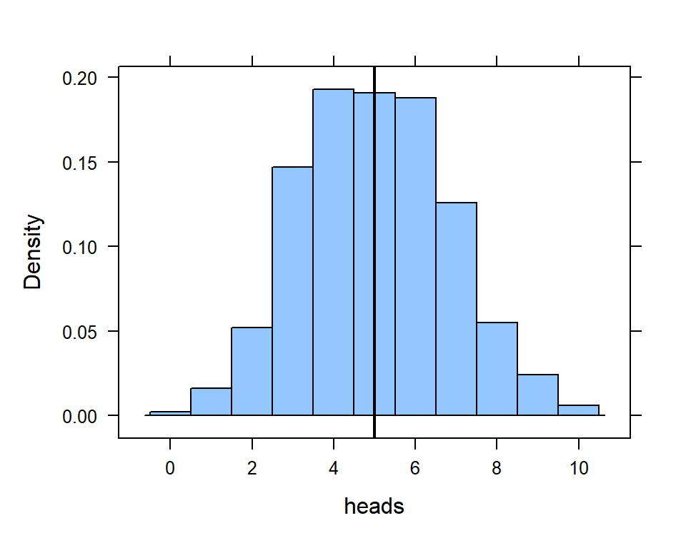
Finally, we might want to look at the likelihood of a particular event happening. In this case, we might want to look at the probability that we would get 9 or more heads (out of 15).
histogram(~heads, data=game.trials, v=9, groups = (heads >= 9))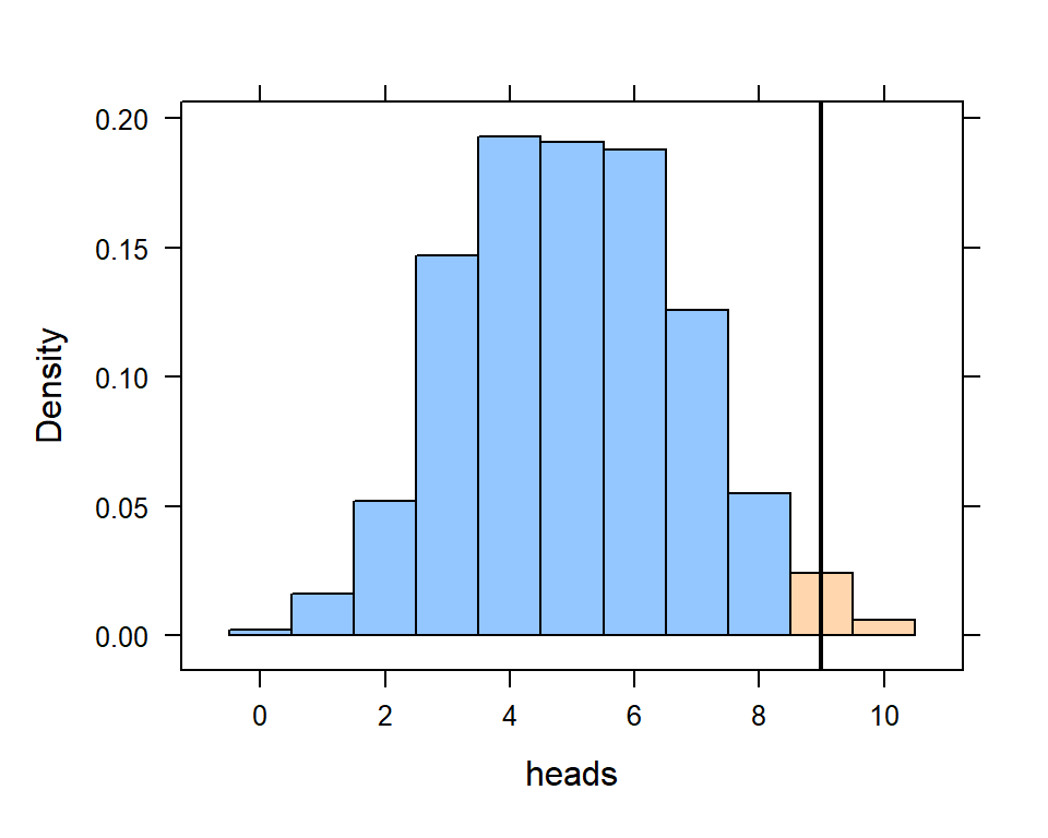
Remember that this histogram is a visual representation of the distribution of the 1000 trials of flipping 15 coins. By using the groups = (heads >= 9) argument, we can see the blue group (less than 9 heads) and the pink group (9 or more heads).
4.5 Functions - sampling
4.5.1 Simple Random Sampling
Let’s say you are doing an experiment and you want to use simple random sampling to select your subjects. We can use the ‘sample()’ function as follows:
# Generate 25 random numbers between 1 and 100:
sample(1:99, 25, replace = FALSE)
## [1] 8 38 31 36 26 83 48 30 90 68 2 42 92 1 95 6 4 41 86 39 32 49 25 15 61Note that we use the ‘replace=FALSE’ argument to ensure that we don’t pick the same subject twice.
4.5.2 Randomizing subjects into treatment groups.
To randomize subjects into treatment groups, we can also use the ‘sample()’ function, but with replacement (‘replace=TRUE’).
# Randomize 25 patients into two groups - Control (0) and Treatment (1)
sample(0:1, 25, replace = TRUE)
## [1] 0 1 1 0 1 0 1 1 0 0 1 0 1 1 0 1 1 1 0 1 0 1 1 0 04.5.3 Random sample and treatment groups
Let’s put both of the above things together into one algorighm. Let’s say that we have a sampling frame of 100 subjects and we want to pick 12 subjects, with exactly 3 subjects in each of 4 treatment groups. We use the ‘set.seed()’ function to ensure reproducibility - that is, so we always get the same sample from the following code.
samplesize <- 12
framesize <- 100
numgroups <- 4

set.seed(201)

# Let's set up the groups to be the same size
subjects <- samplesize / numgroups
groups <- c(rep("A",subjects), rep("B", subjects), rep("C", subjects), rep("D", subjects))

(mysample <- data.table(house = sample(1:framesize, samplesize, rep = FALSE),
                       group = sample(groups, samplesize, rep = FALSE)))
## house group
## 1: 83 A
## 2: 54 B
## 3: 42 B
## 4: 49 D
## 5: 5 B
## 6: 37 C
## 7: 89 C
## 8: 7 D
## 9: 62 A
## 10: 99 C
## 11: 25 D
## 12: 56 AWe can use the 'tally()' and 'arrange()' commands to check that our sample is correct. tally(~group, data=mysample)## group
## A B C D
## 3 3 3 3arrange(mysample, group, house)## house group
## 1: 56 A
## 2: 62 A
## 3: 83 A
## 4: 5 B
## 5: 42 B
## 6: 54 B
## 7: 37 C
## 8: 89 C
## 9: 99 C
## 10: 7 D
## 11: 25 D
## 12: 49 D