14 Power Analysis

O ne of the reasons why meta-analysis can be so helpful is because it allows us to combine several imprecise findings into a more precise one. In most cases, meta-analyses produce estimates with narrower confidence intervals than any of the included studies. This is particularly useful when the true effect is small. While primary studies may not be able to ascertain the significance of a small effect, meta-analytic estimates can often provide the statistical power needed to verify that such a small effect exists.
Lack of statistical power, however, may still play an important role–even in meta-analysis. The number of included studies in many meta-analyses is small, often below \(K=\) 10. The median number of studies in Cochrane systematic reviews, for example, is six (Borenstein et al. 2011). This becomes even more problematic if we factor in that meta-analyses often include subgroup analyses and meta-regression, for which even more power is required. Furthermore, many meta-analyses show high between-study heterogeneity. This also reduces the overall precision and thus the statistical power.
We already touched on the concept of statistical power in Chapter 9.2.2.2, where we learned about the p-curve method. The idea behind statistical power is derived from classical hypothesis testing. It is directly related to the two types of errors that can occur in a hypothesis test. The first error is to accept the alternative hypothesis (e.g. \(\mu_1 \neq \mu_2\)) while the null hypothesis (\(\mu_1 = \mu_2\)) is true. This leads to a false positive, also known as a Type I or \(\alpha\) error. Conversely, it is also possible that we accept the null hypothesis, while the alternative hypothesis is true. This generates a false negative, known as a Type II or \(\beta\) error.
The power of a test directly depends on \(\beta\). It is defined as Power = \(1 - \beta\). Suppose that our null hypothesis states that there is no difference between the means of two groups, while the alternative hypothesis postulates that a difference (i.e. an “effect”) exists. The statistical power can be defined as the probability that the test will detect an effect (i.e. a mean difference), if it exists:
\[\begin{equation} \text{Power} = P(\text{reject H}_0~|~\mu_1 \neq \mu_2) = 1 - \beta \tag{14.1} \end{equation}\]
It is common practice to assume that a type I error is more grave than a type II error. Thus, the \(\alpha\) level is conventionally set to 0.05 and the \(\beta\) level to 0.2. This leads to a threshold of \(1-\beta\) = 1 - 0.2 = 80%, which is typically used to determine if the statistical power of a test is adequate or not. When researchers plan a new study, they usually select a sample size that guarantees a power of 80%. It is easier to obtain statistically significant results when the true effect is large. Therefore, when the power is fixed at 80%, the required sample size only depends on the size of the true effect. The smaller the assumed effect, the larger the sample size needed to ascertain 80% power.
Researchers who conduct a primary study can plan the size of their sample a priori, based on the effect size they expect to find. The situation is different in meta-analysis, where we can only work with the published material. However, we have some control over the number and type of studies we include in our meta-analysis (e.g. by defining more lenient or strict inclusion criteria). This way, we can also adjust the overall power. There are several factors that can influence the statistical power in meta-analyses:
The total number of included or eligible studies, and their sample size. How many studies do we expect, and are they rather small or large?
The effect size we want to find. This is particularly important, as we have to make assumptions about how big an effect size has to be to still be meaningful. For example, one study calculated that for depression interventions, even effects as small as SMD = 0.24 may still be meaningful to patients (Pim Cuijpers et al. 2014). If we want to study negative effects of an intervention (e.g. death or symptom deterioration), even very small effect sizes are extremely important and should be detected.
The expected between-study heterogeneity. Substantial heterogeneity affects the precision of our meta-analytic estimates, and thus our potential to find significant effects.
Besides that, it is also important to think about other analyses, such as subgroup analyses, that we want to conduct. How many studies are there for each subgroup? What effects do we want to find in each group?
Post-Hoc Power Tests: “The Abuse of Power”
Please note that power analyses should always be conducted a priori, meaning before you perform the meta-analysis.
Power analyses conducted after an analysis (“post-hoc”) are based on a logic that is deeply flawed (Hoenig and Heisey 2001). First, post-hoc power analyses are uniformative–they tell us nothing that we do not already know. When we find that an effect is not significant based on our collected sample, the calculated post-hoc power will be, by definition, insufficient (i.e. 50% or lower). When we calculate the post-hoc power of a test, we simply “play around” with a power function that is directly linked to the \(p\)-value of the result.
There is nothing in the post-hoc power estimate that the \(p\)-value would not already tell us. Namely that, based on the effect and sample size of our test, the power is insufficient to ascertain statistical significance.
When we interpret the post-hoc power, this can also lead to the power approach paradox (PAP). This paradox arises because an analysis yielding no significant effect is thought to show more evidence that the null hypothesis is true when the p-value is smaller, since then, the power to detect a true effect would be higher.
14.1 Fixed-Effect Model
To determine the power of a meta-analysis under the fixed-effect model, we have to specify a distribution which represents that our alternative hypothesis is correct. To do this, however, it is not sufficient to simply say that \(\theta \neq 0\) (i.e. that some effect exists). We have to assume a specific true effect that we want to be able to detect with sufficient (80%) power. For example SMD = 0.29.
We already covered previously (see Chapter 8.1.2) that dividing an effect size through its standard error creates a \(z\) score. These \(z\) scores follow a standard normal distribution, where a value of \(|z| \geq\) 1.96 means that the effect is significantly different from zero (\(p<\) 0.05). This is exactly what we want to achieve in our meta-analysis: no matter how large the exact effect size and standard error of our result, the value of \(|z|\) should be at least 1.96, and thus statistically significant:
\[\begin{equation} z = \frac{\theta}{\sigma_{\theta}}~~~\text{where}~~~|z| \geq 1.96. \tag{14.2} \end{equation}\]
The value of \(\sigma_{\theta}\), the standard error of the pooled effect size, can be calculated using this formula:
\[\begin{equation} \sigma_{\theta}=\sqrt{\frac{\left(\frac{n_1+n_2}{n_1n_2}\right)+\left(\frac{\theta^2}{2(n_1+n_2)}\right)}{K}} \tag{14.3} \end{equation}\]
Where \(n_1\) and \(n_2\) stand for the sample sizes in group 1 and group 2 of a study, where \(\theta\) is the assumed effect size (expressed as a standardized mean difference), and \(K\) is the total number of studies in our meta-analysis. Importantly, as a simplification, this formula assumes that the sample sizes in both groups are identical across all included studies.
The formula is very similar to the one used to calculate the standard error of a standardized mean difference, with one exception. We now divide the the standard error by \(K\). This means that the standard error of our pooled effect is reduced by factor \(K\), representing the total number of studies in our meta-analysis. Put differently, when assuming a fixed-effect model, pooling the studies leads to a \(K\)-fold increase in the precision of our overall effect76.
After we defined \(\theta\) and calculated \(\sigma_{\theta}\), we end up with a value of \(z\). This \(z\) score can be used to obtain the power of our meta-analysis, given a number of studies \(K\) with group sizes \(n_1\) and \(n_2\):
\[\begin{align} \text{Power} &= 1-\beta \notag \\ &= 1-\Phi(c_{\alpha}-z)+\Phi(-c_{\alpha}-z) \notag \\ &= 1-\Phi(1.96-z)+\Phi(-1.96-z). \tag{14.4} \end{align}\]
Where \(c_{\alpha}\) is the critical value of the standard normal distribution, given a specified \(\alpha\) level. The \(\Phi\) symbol represents the cumulative distribution function (CDF) of a standard normal distribution, \(\Phi(z)\). In R, the CDF of the standard normal distribution is implemented in the pnorm function.
We can now use these formulas to calculate the power of a fixed-effect meta-analysis. Imagine that we expect \(K=\) 10 studies, each with approximately 25 participants in both groups. We want to be able to detect an effect of SMD = 0.2. What power does such a meta-analysis have?
# Define assumptions
theta <- 0.2
K <- 10
n1 <- 25
n2 <- 25

# Calculate pooled effect standard error
sigma <- sqrt(((n1+n2)/(n1*n2)+(theta^2/(2*n1+n2)))/K)

# Calculate z
z = theta/sigma

# Calculate the power
1 - pnorm(1.96-z) + pnorm(-1.96-z)
## [1] 0.6059151We see that, with 60.6%, such a meta-analysis would be underpowered, even though 10 studies were included. A more convenient way to calculate the power of a (fixed-effect) meta-analysis is to use the power.analysis function.
The power.analysis function contains these arguments:
d. The hypothesized, or plausible overall effect size, expressed as the standardized mean difference (SMD). Effect sizes must be positive numeric values.OR. The assumed effect of a treatment or intervention compared to control, expressed as an odds ratio (OR). If bothdandORare specified, results will only be computed for the value ofd.k. The expected number of studies included in the meta-analysis.n1,n2. The expected average sample size in group 1 and group 2 of the included studies.p. The alpha level to be used. Default is \(\alpha\)=0.05.heterogeneity. The level of between-study heterogeneity. Can either be"fixed"for no heterogeneity (fixed-effect model),"low"for low heterogeneity,"moderate"for moderate-sized heterogeneity, or"high"for high levels of heterogeneity. Default is"fixed".
Let us try out this function, using the same input as in the example from before.
library(dmetar)
power.analysis(d = 0.2,
               k = 10,
               n1 = 25,
               n2 = 25,
               p = 0.05)
## Fixed-effect model used.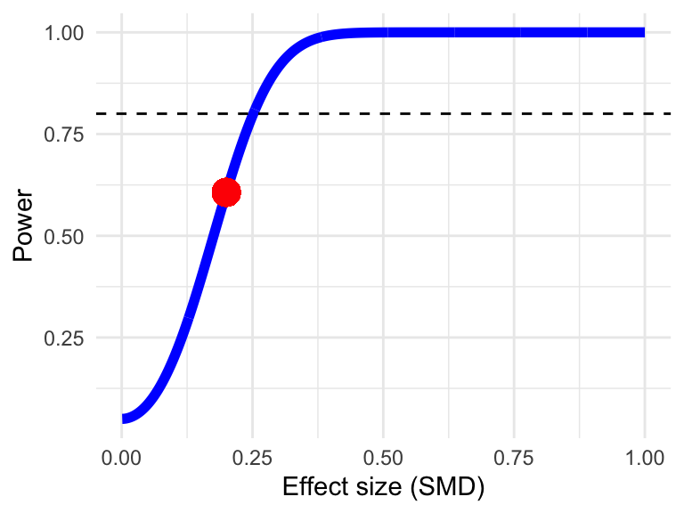
## Power: 60.66%14.2 Random-Effects Model
For power analyses assuming a random-effects model, we have to take the between-study heterogeneity variance \(\tau^2\) into account. Therefore, we need to calculate an adapted version of the standard error, \(\sigma^*_{\theta}\):
\[\begin{equation} \sigma^*_{\theta}=\sqrt{\frac{\left(\frac{n_1+n_2}{n_1n_2}\right)+\left(\frac{\theta^2}{2(n_1+n_2)}\right)+\tau^2}{K}} \tag{14.5} \end{equation}\]
The problem is that the value of \(\tau^2\) is usually not known before seeing the data. Hedges and Pigott (2001), however, provide guidelines that may be used to model either low, moderate or large between-study heterogeneity:
Low heterogeneity:
\[\begin{equation} \sigma^*_{\theta} = \sqrt{1.33\times\dfrac{\sigma^2_{\theta}}{K}} \tag{14.6} \end{equation}\]
Moderate heterogeneity:
\[\begin{equation} \sigma^*_{\theta} = \sqrt{1.67\times\dfrac{\sigma^2_{\theta}}{K}} \tag{14.7} \end{equation}\]
Large heterogeneity:
\[\begin{equation} \sigma^*_{\theta} = \sqrt{2\times\dfrac{\sigma^2_{\theta}}{K}} \tag{14.8} \end{equation}\]
The power.analysis function can also be used for random-effects meta-analyses. The amount of assumed between-study heterogeneity can be controlled using the heterogeneity argument. Possible values are "low", "moderate" and "high". Using the same values as in the previous example, let us now calculate the expected power when the between-study heterogeneity is moderate.
power.analysis(d = 0.2,
               k = 10,
               n1 = 25,
               n2 = 25,
               p = 0.05,
               heterogeneity = "moderate")
## Random-effects model used (moderate heterogeneity assumed).
## Power: 40.76%We see that the estimated power is 40.76%. This is lower than the normative 80% threshold. It is also lower than the 60.66% we obtain we assuming a fixed-effect model. This is because between-study heterogeneity decreases the precision of our pooled effect estimate, resulting in a drop in statistical power.
Figure 14.1 visualizes the effect of the true effect size, number of studies, and amount of between-study heterogeneity on the power of a meta-analysis.77
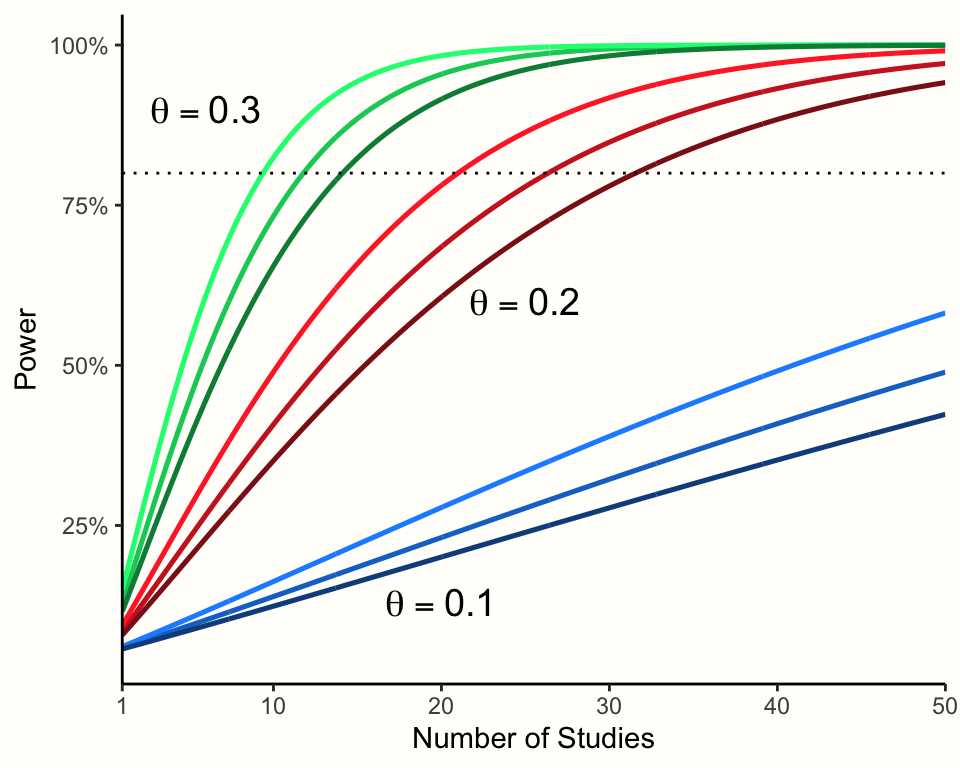
Figure 14.1: Power of random-effects meta-analyses (\(n\)=50 in each study). Darker colors indicate higher between-study heterogeneity.
14.3 Subgroup Analyses
When planning subgroup analyses, it can be relevant to know how large the difference between two groups must be so that we can detect it, given the number of studies at our disposal. This is where a power analysis for subgroup differences can be applied. A subgroup power analysis can be conducted in R using the power.analysis.subgroup function, which implements an approach described by Hedges and Pigott (2004).
Let us assume that we expect the first group to show an effect of SMD = 0.3 with a standard error of 0.13, while the second group has an effect of SMD = 0.66, and a standard error of 0.14. We can use these assumptions as input to our call to the function:
power.analysis.subgroup(TE1 = 0.30, TE2 = 0.66,
                        seTE1 = 0.13, seTE2 = 0.14)
## Minimum effect size difference needed for sufficient power: 0.536 (input: 0.36)
## Power for subgroup difference test (two-tailed): 46.99%
In the output, we can see that the power of our imaginary subgroup test (47%) would not be sufficient. The output also tells us that, all else being equal, the effect size difference needs to be at least 0.54 in order to reach sufficient power.
\[\tag*{$\blacksquare$}\]