10 “Multilevel” Meta-Analysis

W elcome to the advanced methods section. In the previous part of the guide, we took a deep dive into topics that we consider highly relevant for almost every meta-analysis. With this background, we can now proceed to somewhat more advanced techniques.
We consider the following methods “advanced” because their mathematical underpinnings are more involved, or because of their implementation in R. However, if you have worked yourself through the previous chapters of the guide, you should be more than well equipped to understand and implement the contents that are about to follow. Many of the following topics merit books of their own, and what we cover here should only be considered as a brief introduction. Where useful, we will therefore also provide literature for further reading.
This first chapter deals with the topic of “multilevel” meta-analyses. You probably wonder why we put the word “multilevel” into quotation marks. Describing a study as a “multilevel” meta-analysis insinuates that this is something special or extraordinary compared to “standard” meta-analyses.
Yet, that is not true. Every meta-analytic model presupposes a multilevel structure of our data to pool results (Pastor and Lazowski 2018). In the chapters before, we have already fitted a multilevel (meta-analysis) model several times–without even knowing.
When people talk about multilevel meta-analysis, what they think of are three-level meta-analysis models. Such models are indeed somewhat different to the fixed-effect and random-effects model we already know. In this chapter, we will therefore first describe why meta-analysis naturally implies a multilevel structure of our data, and how we can extend a conventional meta-analysis to a three-level model. As always, we will also have a look at how such models can be fitted in R using a hands-on example.
10.1 The Multilevel Nature of Meta-Analysis
To see why meta-analysis has multiple levels by default, let us go back to the formula of the random-effects model that we discussed in Chapter 4.1.2:
\[\begin{equation} \hat\theta_k = \mu + \epsilon_k + \zeta_k \tag{10.1} \end{equation}\]
We discussed that the terms \(\epsilon_k\) and \(\zeta_k\) are introduced in a random-effects model because we assume that there are two sources of variability. The first one is caused by the sampling error (\(\epsilon_k\)) of individual studies, which leads effect size estimates to deviate from the true effect size \(\theta_k\).
The second one, \(\zeta_k\), represents the between-study heterogeneity. This heterogeneity is caused by the fact that the true effect size of some study \(k\) is again only part of an overarching distribution of true effect sizes. This distribution is from where the individual true effect size \(\theta_k\) was drawn. Therefore, our aim in the random-effects model is to estimate the mean of the distribution of true effect sizes, denoted with \(\mu\).
The two error terms \(\epsilon_k\) and \(\zeta_k\) correspond with the two levels in our meta-analysis data: the “participant” level (level 1) and the “study” level (level 2). Figure 10.1 below symbolizes this structure.
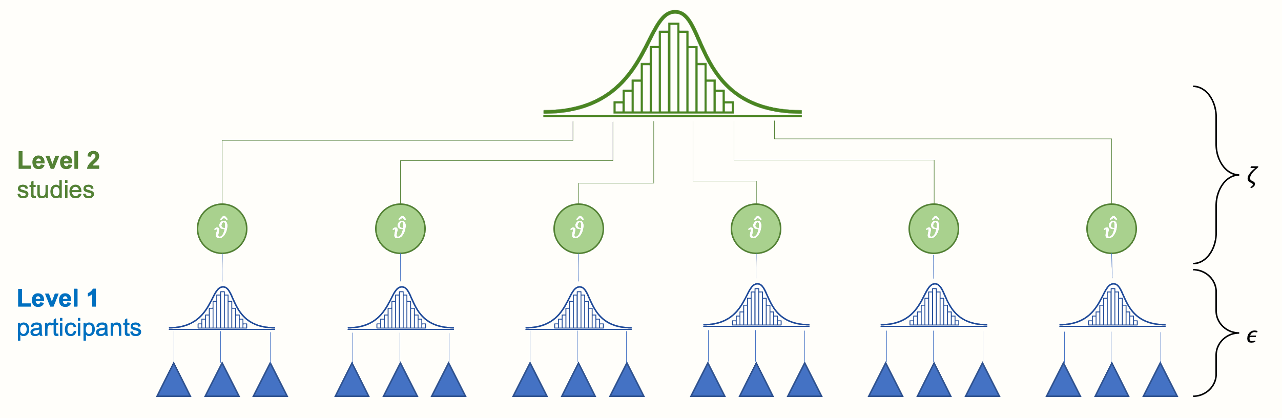
Figure 10.1: Multilevel structure of the conventional random-effects model.
At the lowest level (level 1) we have the participants (or patients, specimens, etc., depending on the research field). These participants are part of larger units: the studies included in our meta-analysis. This overlying layer of studies constitutes our second level.
When we conduct a meta-analysis, data on level 1 usually already reaches us in a “pooled” form (e.g. the authors of the paper provide us with the mean and standard deviation of their studied sample instead of the raw data). Pooling on level 2, the study level, however, has to be performed as part of the meta-analysis. Traditionally, such type of data is called nested: one can say that participants are “nested” within studies.
Let us go back to the random-effects model formula in equation (10.1). Implicitly, this formula already describes the multilevel structure of our meta-analysis data. To make this more obvious, we have to split the equation into two formulas, where each corresponds to one of the two levels. If we do this, we get the following result:
Level 1 (participants) model:
\[\begin{equation} \hat\theta_k = \theta_k + \epsilon_k \tag{10.2} \end{equation}\]
Level 2 (studies) model:
\[\begin{equation} \theta_k = \mu + \zeta_k \tag{10.3} \end{equation}\]
You might have already detected that we can substitute \(\theta_k\) in the first equation with its definition in the second equation. What we then obtain is a formula exactly identical to the one of the random-effects model from before. The fixed-effects model can also be written in this way–we only have to set \(\zeta_k\) to zero. Evidently, our plain old meta-analysis model already has multilevel properties “built in”. It exhibits this property because we assume that participants are nested within studies in our data.
This makes it clear that meta-analysis naturally possesses a multilevel structure. It is possible to expand this structure even further in order to better capture certain mechanisms that generated our data. This is where three-level models (Cheung 2014; Assink, Wibbelink, et al. 2016) come into play.
Statistical independence is one of the core assumptions when we pool effect sizes in a meta-analysis. If there is a dependency between effect sizes (i.e. effect sizes are correlated), this can artificially reduce heterogeneity and thus lead to false-positive results. This issue is known as the unit-of-analysis error, which we already covered before (see Chapter 3.5.2). Effect size dependence can stem from different sources (Cheung 2014):
Dependence introduced by the authors of the individual studies. For example, scientists conducting the study may have collected data from multiple sites, compared multiple interventions to one single control group, or used different questionnaires to measure the same outcome. In all of these scenarios, we can assume that some kind of dependency is introduced within the reported data.
Dependence introduced by the meta-analyst herself. As an example, think of a meta-analysis that focuses on some psychological mechanism. This meta-analysis includes studies which were conducted in different cultural regions of the world (e.g. East Asian and Western European societies). Depending on the type of psychological mechanism, it could be that results of studies conducted in the same cultural region are more similar compared to those conducted in a different culture.
We can take such dependencies into account by integrating a third layer into the structure of our meta-analysis model. For example, one could model that effect sizes based on different questionnaires are nested within studies. Or one could create a model in which studies are nested within cultural regions. This creates a three-level meta-analysis model, as illustrated by the next figure.
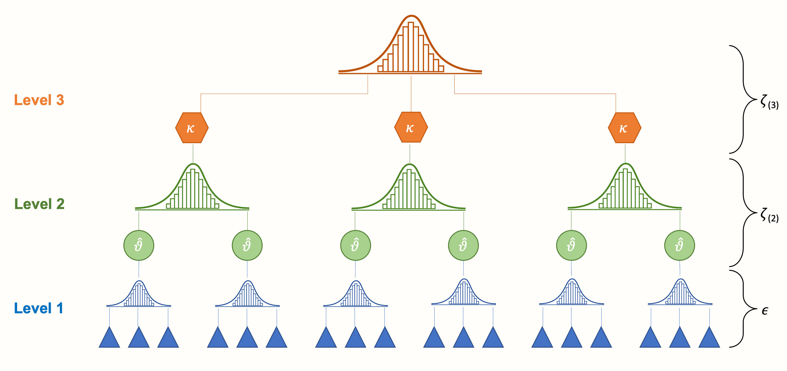
We see that a three-level model contains three pooling steps. First, researchers themselves “pool” the results of individual participants in their primary studies, and report the aggregated effect size. Then, on level 2, these effect sizes are nested within several clusters, denoted by \(\kappa\). These cluster can either be individual studies (i.e. many effect sizes are nested in one study), or subgroups of studies (i.e. many studies are nested in one subgroup, where each study contributes only one effect size).
Lastly, pooling the aggregated cluster effects leads to the overall true effect size \(\mu\). Conceptually, this average effect is very close to the pooled true effect \(\mu\) in a fixed- or random-effects model. The difference, however, is that it is based on a model in which we explicitly account for dependent effect sizes in our data.
It is possible to write down the formula of the three-level model using the same level notation we used before. The greatest distinction is that now, we need to define three formulas instead of two:
Level 1 model:
\[\begin{equation} \hat\theta_{ij} = \theta_{ij} + \epsilon_{ij} \tag{10.4} \end{equation}\]
Level 2 model:
\[\begin{equation} \theta_{ij} = \kappa_{j} + \zeta_{(2)ij} \tag{10.5} \end{equation}\]
Level 3 model:
\[\begin{equation} \kappa_{j} = \mu + \zeta_{(3)j} \tag{10.6} \end{equation}\]
Where \(\hat\theta_{ij}\) is an estimate of the true effect size \(\theta_{ij}\). The term \(ij\) can be read as “some effect size \(i\) nested in cluster \(j\)”. Parameter \(\kappa_{j}\) is the average effect size in cluster \(j\), and \(\mu\) the overall average population effect. Like before, we can piece these formulas together and thus reduce the formula to one line:
\[\begin{equation} \hat\theta_{ij} = \mu + \zeta_{(2)ij} + \zeta_{(3)j} + \epsilon_{ij} \tag{10.7} \end{equation}\]
We see that, in contrast to the random-effects model, this formula now contains two heterogeneity terms. One is \(\zeta_{(2)ij}\), which stands for the within-cluster heterogeneity on level 2 (i.e. the true effect sizes within cluster \(j\) follow a distribution with mean \(\kappa_j\)). The other is \(\zeta_{(3)j}\), the between-cluster heterogeneity on level 3. Consequentially, fitting a three-level meta-analysis model does not only involve the estimation of one heterogeneity variance parameter \(\tau^2\). We have to estimate two \(\tau^2\) values: one for level 2, and the other for level 3.
The {metafor} package is particularly well suited for fitting meta-analytic three-level models. It uses (restricted) maximum likelihood procedures to do so. Previously, we primarily used functions of the {meta} package to run meta-analyses. We did this because this package is a little less technical, and thus better suited for beginners. Yet, the {metafor} package, as we have seen in Chapter 8.3.3, is also fairly easy to use once the data is prepared correctly. How exactly one can use {metafor} to fit three-level models in R will be the topic of the next section50.
10.2 Fitting Three-Level Meta-Analysis Models in R
As mentioned before, we need the {metafor} package to fit three-level meta-analysis models. Therefore, we need to load it from our library first.
In our hands-on example, we will use the Chernobyl data set. This data set is loosely based on a real meta-analysis which examined the correlation between ionizing radiation (“nuclear fallout”) and mutation rates in humans, caused by the devastating 1986 Chernobyl reactor disaster (Møller and Mousseau 2015).
To see the general structure of the data, we can use the head function. This prints the first six rows of the data frame that we just loaded into our global environment.
head(Chernobyl)## author cor n z se.z var.z radiation es.id
## 1 Aghajanyan & Suskov (2009) 0.20 91 0.20 0.10 0.01 low id_1
## 2 Aghajanyan & Suskov (2009) 0.26 91 0.27 0.10 0.01 low id_2
## 3 Aghajanyan & Suskov (2009) 0.20 92 0.20 0.10 0.01 low id_3
## 4 Aghajanyan & Suskov (2009) 0.26 92 0.27 0.10 0.01 low id_4
## 5 Alexanin et al. (2010) 0.93 559 1.67 0.04 0.00 low id_5
## 6 Alexanin et al. (2010) 0.44 559 0.47 0.04 0.00 low id_6The data set contains eight columns. The first one, author, displays the name of the study. The cor column shows the (un-transformed) correlation between radiation exposure and mutation rates, while n stands for the sample size. The columns z, se.z, and var.z are the Fisher-\(z\) transformed correlations (Chapter 3.2.3.1), as well their standard error and variance. The radiation column serves as a moderator, dividing effect sizes into subgroups with low and high overall radiation exposure. The es.id column simply contains a unique ID for each effect size (i.e. each row in our data frame).
A peculiar thing about this data set is that it contains repeated entries in author. This is because most studies in this meta-analysis contributed more than one observed effect size. Some studies used several methods to measure mutations or several types of index persons (e.g. exposed parents versus their offspring), all of which leads to multiple effects per study.
Looking at this structure, it is quite obvious that effect sizes in our data set are not independent. They follow a nested structure, where various effect sizes are nested in one study. Thus, it might be a good idea to fit a three-level meta-analysis in order to adequately model these dependencies in our data.
10.2.1 Model Fitting
A three-level meta-analysis model can be fitted using the rma.mv function in {metafor}. Here is a list of the most important arguments for this function, and how they should be specified:
yi. The name of the column in our data set which contains the calculated effect sizes. In our example, this isz, since Fisher-\(z\) transformed correlations have better mathematical properties than “untransformed” correlations.V. The name of the column in our data set which contains the variance of the calculated effect sizes. In our case, this isvar.z. It is also possible to use the squared standard error of the effect size, since \(SE_k^2 = v_k\).slab. The name of the column in our data set which contains the study labels, similar tostudlabin {meta}.data. The name of the data set.test. The test we want to apply for our regression coefficients. We can choose from"z"(default) and"t"(recommended; uses a test similar to the Knapp-Hartung method).method. The method used to estimate the model parameters. Both"REML"(recommended; restricted maximum-likelihood) and"ML"(maximum likelihood) are possible. Please note that other types of between-study heterogeneity estimators (e.g. Paule-Mandel) are not applicable here.
The most important argument, however, is random. Arguably, it is also the trickiest one. In this argument, we specify a formula which defines the (nested) random effects. For a three-level model, the formula always starts with ~ 1, followed by a vertical bar |. Behind the vertical bar, we assign a random effect to a grouping variable (such as studies, measures, regions, etc.). This grouping variable is often called a random intercept because it tells our model to assume different effects (i.e. intercepts) for each group.
In a three-level model, there are two grouping variables: one on level 2, and another on level 3. We assume that these grouping variables are nested: several effects on level 2 together make up a larger cluster on level 3.
There is a special way through which we can tell rma.mv to assume such nested random effects. We do this using a slash (/) to separate the higher- and lower-level grouping variable. To the left of /, we put in the level 3 (cluster) variable. To the right, we insert the lower-order variable nested in the larger cluster. Therefore, the general structure of the formula looks like this: ~ 1 | cluster/effects_within_cluster.
In our example, we assume that individual effect sizes (level 2; defined by es.id) are nested within studies (level 3; defined by author). This results in the following formula: ~ 1 | author/es.id. The complete rma.mv function call looks like this:
full.model <- rma.mv(yi = z,
                     V = var.z,
                     slab = author,
                     data = Chernobyl,
                     random = ~ 1 | author/es.id,
                     test = "t",
                     method = "REML")
We gave the output the name full.model. To print an overview of the results, we can use the summary function.
summary(full.model)## Multivariate Meta-Analysis Model (k = 33; method: REML)
## [...]
## Variance Components:
##
## estim sqrt nlvls fixed factor
## sigma^2.1 0.1788 0.4229 14 no author
## sigma^2.2 0.1194 0.3455 33 no author/es.id
##
## Test for Heterogeneity:
## Q(df = 32) = 4195.8268, p-val < .0001
##
## Model Results:
##
## estimate se tval pval ci.lb ci.ub
## 0.5231 0.1341 3.9008 0.0005 0.2500 0.7963 ***
## [...]First, have a look at the Variance Components. Here, we see the random-effects variances calculated for each level of our model. The first one, sigma^2.1, shows the level 3 between-cluster variance. In our example, this is equivalent to the between-study heterogeneity variance \(\tau^2\) in a conventional meta-analysis (since clusters represent studies in our model).
The second variance component sigma^2.2 shows the variance within clusters (level 2). In the nlvls column, we see the number of groups on each level. Level 3 has 14 groups, equal to the \(K=\) 14 included studies. Together, these 14 studies contain 33 effect sizes, as shown in the second row.
Under Model Results, we see the estimate of our pooled effect, which is \(z=\) 0.52 (95%CI: 0.25–0.80). To facilitate the interpretation, it is advisable to transform the effect back to a normal correlation. This can be done using the convert_z2r function in the {esc} package:
library(esc)
convert_z2r(0.52)
## [1] 0.4777We see that this leads to a correlation of approximately \(r \approx\) 0.48. This can be considered large. There seems to be a substantial association between mutation rates and exposure to radiation from Chernobyl.
The Test for Heterogeneity in the output points at true effect size differences in our data (\(p<\) 0.001). This result, however, is not very informative. We are more interested in the precise amount of heterogeneity variance captured by each level in our model. It would be good to know how much of the heterogeneity is due to differences within studies (level 2), and how much is caused by between-study differences (level 3).
10.2.2 Distribution of Variance Across Levels
We can answer this question by calculating a multilevel version of \(I^2\) (Cheung 2014). In conventional meta-analyses, \(I^2\) represents the amount of variation not attributable to sampling error (see Chapter 5.1.2; i.e. the between-study heterogeneity). In three-level models, this heterogeneity variance is split into two parts: one attributable to true effect size differences within clusters, and the other to between-cluster variation. Thus, there are two \(I^2\) values, quantifying the percentage of total variation associated with either level 2 or level 3.
The var.comp function only needs a fitted rma.mv model as input. We save the output in i2 and then use the summary function to print the results.
##         % of total variance    I2
## Level 1            1.254966   ---
## Level 2           39.525499 39.53
## Level 3           59.219534 59.22
## Total I2: 98.75%
In the output, we see the percentage of total variance attributable to each of the three levels. The sampling error variance on level 1 is very small, making up only roughly 1%. The value of \(I^2_{\text{Level 2}}\), the amount of heterogeneity variance within clusters, is much higher, totaling roughly 40%. The largest share, however, falls to level 3. Between-cluster (here: between-study) heterogeneity makes up \(I^2_{\text{Level 3}}=\) 59% of the total variation in our data.
Overall, this indicates that there is substantial between-study heterogeneity on the third level. Yet, we also see that a large proportion of the total variance, more than one third, can be explained by differences within studies.
It is also possible to visualize this distribution of the total variance. We only have to plug the var.comp output into the plot function.
plot(i2)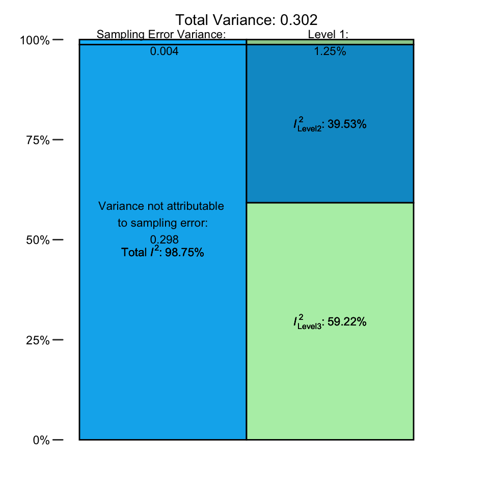
10.2.3 Comparing Models
Fitting a three-level model only makes sense when it represents the variability in our data better than a two-level model. When we find that a two-level model provides a fit comparable to a three-level model, Occam’s razor should be applied: we favor the two-level model over the three-level model, since it is less complex, but explains our data just as well.
Fortunately, the {metafor} package makes it possible to compare our three-level model to one in which a level is removed. To do this, we use the rma.mv function again; but this time, set the variance component of one level to zero. This can be done by specifying the sigma2 parameter. We have to provide a vector with the generic form c(level 3, level 2). In this vector, we fill in 0 when a variance component should be set to zero, while using NA to indicate that a parameter should be estimated from the data.
In our example, it makes sense to check if nesting individual effect sizes in studies has improved our model. Thus, we fit a model in which the level 3 variance, representing the between-study heterogeneity, is set to zero. This is equal to fitting a simple random-effects model in which we assume that all effect sizes are independent (which we know they are not). Since level 3 is held constant at zero, the input for sigma2 is c(0, NA). This results in the following call to rma.mv, the output of which we save under the name l3.removed.
l3.removed <- rma.mv(yi = z,
                     V = var.z,
                     slab = author,
                     data = Chernobyl,
                     random = ~ 1 | author/es.id,
                     test = "t",
                     method = "REML",
                     sigma2 =  c(0, NA))

summary(l3.removed)
## [...]
## Variance Components:
##
## estim sqrt nlvls fixed factor
## sigma^2.1 0.0000 0.0000 14 yes author
## sigma^2.2 0.3550 0.5959 33 no author/es.id
##
## Test for Heterogeneity:
## Q(df = 32) = 4195.8268, p-val < .0001
##
## Model Results:
##
## estimate se tval pval ci.lb ci.ub
## 0.5985 0.1051 5.6938 <.0001 0.3844 0.8126 ***
## [...]In the output, we see that sigma^2.1 has been set to zero–just as intended. The overall effect has also changed. But is this result better than the one of the three-level model? To assess this, we can use the anova function to compare both models.
anova(full.model, l3.removed)## df AIC BIC AICc logLik LRT pval QE
## Full 3 48.24 52.64 49.10 -21.12 4195.82
## Reduced 2 62.34 65.27 62.76 -29.17 16.10 <.0001 4195.82We see that the Full (three-level) model, compared to the Reduced one with two levels, does indeed show a better fit. The Akaike (AIC) and Bayesian Information Criterion (BIC) are lower for this model, which indicates favorable performance. The likelihood ratio test (LRT) comparing both models is significant (\(\chi^2_1=\) 16.1, \(p<\) 0.001), and thus points in the same direction.
We can say that, although the three-level model introduces one additional parameter (i.e. it has 3 degrees of freedom instead of 2), this added complexity seems to be justified. Modeling of the nested data structure was probably a good idea, and has improved our estimate of the pooled effect.
However, please note that there are often good reasons to stick with a three-level structure–even when it does not provide a significantly better fit. In particular, it makes sense to keep a three-level model when we think that it is based on a solid theoretical rationale.
When our data contains studies with multiple effect sizes, for example, we know that these effects can not be independent. It thus makes sense to keep the nested model, since it more adequately represents how the data were “generated”. If the results of anova in our example had favored a two-level solution, we would have concluded that effects within studies were largely homogeneous. But we likely would have reported results of the three-level model anyway. This is because we know that a three-level model represents the data-generating process better.
The situation is somewhat different when the importance of the cluster variable is unclear. Imagine, for example, that clusters on level 3 represent different cultural regions in a three-level model. When we find that the phenomenon under study shows no variation between cultures, it is perfectly fine to drop the third level and use a two-level model instead.
10.3 Subgroup Analyses in Three-Level Models
Once our three-level model is set, it is also possible to assess putative moderators of the overall effect. Previously in this guide, we discovered that subgroup analyses can be expressed as a meta-regression model with a dummy-coded predictor (Chapter 8.1). In a similar vein, we can add regression terms to a “multilevel” model, which leads to a three-level mixed-effects model:
\[\begin{equation} \hat\theta_{ij} = \theta + \beta x_i + \zeta_{(2)ij} + \zeta_{(3)j} + \epsilon_{ij} \tag{10.8} \end{equation}\]
Where \(\theta\) is the intercept and \(\beta\) the regression weight of a predictor variable \(x\). When we replace \(x_i\) with a dummy (Chapter 8.1), we get a model that can be used for subgroup analyses. When \(x\) is continuous, the formula above represents a three-level meta-regression model.
Categorical or continuous predictors can be specified in rma.mv using the mods argument. The argument requires a formula, starting with a tilde (~), and then the name of the predictor. Multiple meta-regression is also possible by providing more than one predictor (e.g. ~ var1 + var2).
In our Chernobyl example, we want to check if correlations differ depending on the overall amount of radiation in the studied sample (low, medium, or high). This information is provided in the radiation column in our data set. We can fit a three-level moderator model using this code:
mod.model <- rma.mv(yi = z, V = var.z,
                    slab = author, data = Chernobyl,
                    random = ~ 1 | author/es.id,
                    test = "t", method = "REML",
                    mods = ~ radiation)

summary(mod.model)
## [...]
## Test of Moderators (coefficients 2:3):
## F(df1 = 2, df2 = 28) = 0.4512, p-val = 0.6414
##
## Model Results:
## estimate se tval pval ci.lb ci.ub
## intrcpt 0.58 0.36 1.63 0.11 -0.14 1.32
## radiationlow -0.19 0.40 -0.48 0.63 -1.03 0.63
## radiationmedium 0.20 0.54 0.37 0.70 -0.90 1.31
## [...]The first important output is the Test of Moderators. We see that \(F_{2, 28}=\) 0.45, with \(p=\) 0.64. This means that there is no significant difference between the subgroups.
The Model Results are printed within a meta-regression framework. This means that we cannot directly extract the estimates in order to obtain the pooled effect sizes within subgroups.
The first value, the intercept (intrcpt), shows the \(z\) value when the overall radiation exposure was high (\(z=\) 0.58). The effect in the low and medium group can be obtained by adding their estimate to the one of the intercept. Thus, the effect in the low radiation group is \(z\) = 0.58 - 0.19 = 0.39, and the one in the medium exposure group is \(z\) = 0.58 + 0.20 = 0.78.
Reporting the Results of Three-Level (Moderator) Models
When we report the results of a three-level model, we should at least mention the estimated variance components alongside the pooled effect. The rma.mv function denotes the random-effects variance on level 3 and 2 with \(\sigma^2_1\) and \(\sigma^2_2\), respectively.
When we report the estimated variance, however, using \(\tau^2_{\text{Level 3}}\) and \(\tau^2_{\text{Level 2}}\) may be preferable since this makes it clear that we are dealing with variances of true (study) effects (i.e. heterogeneity variance). Adding the multilevel \(I^2\) values also makes sense, since they are easier for others to interpret–provided we first explain what they represent.
When you conducted a model comparison using anova, you may at least report the results of the likelihood ratio test. Results of moderator analyses can be reported in a table such as the one presented in Chapter 7.3. Here is one way to report the results in our example:
“The pooled correlation based on the three-level meta-analytic model was \(r=\) 0.48 (95%CI: 0.25-0.66; \(p\) < 0.001). The estimated variance components were \(\tau^2_{\text{Level 3}}=\) 0.179 and \(\tau^2_{\text{Level 2}}=\) 0.119. This means that \(I^2_{\text{Level 3}}=\) 58.22% of the total variation can be attributed to between-cluster, and \(I^2_{\text{Level 2}}=\) 31.86% to within-cluster heterogeneity. We found that the three-level model provided a significantly better fit compared to a two-level model with level 3 heterogeneity constrained to zero (\(\chi^2_1=\) 16.10; \(p\)< 0.001).”
10.4 Robust Variance Estimation
In the last chapters, we introduced three-level meta-analytic models, and how they can be used to model dependencies between effect sizes in our data. The hierarchical model that we fitted before clearly provides a better representation of our data set than a “conventional” meta-analysis, which assumes that all effect sizes are completely independent. But it is still a simplification of reality. In practice, there are often forms of dependence between effect sizes that are more complex than what is currently captured by our nested model.
We already see this when we go back to our Chernobyl data set. In the data, most studies provide more than one effect size, but the reason for this differs between studies. Some studies compared the effect of radiation in different target populations, and therefore reported more than one effect size. Others used different methods on the same sample, which also means that the study provides more than one effect size.
When several effect sizes in one study are based on the same sample, we expect their sampling errors (the \(\epsilon_{ij}\) terms in equation 10.7 and 10.8 in Chapters 10.1 and 10.3, respectively) to be correlated. This, however, is not yet captured by our three-level model. Our model above assumes that, within clusters/studies, the correlation (and thus the covariance) between sampling errors is zero. Or, to put it differently, it assumes that, within one cluster or study, effect size estimates are independent.
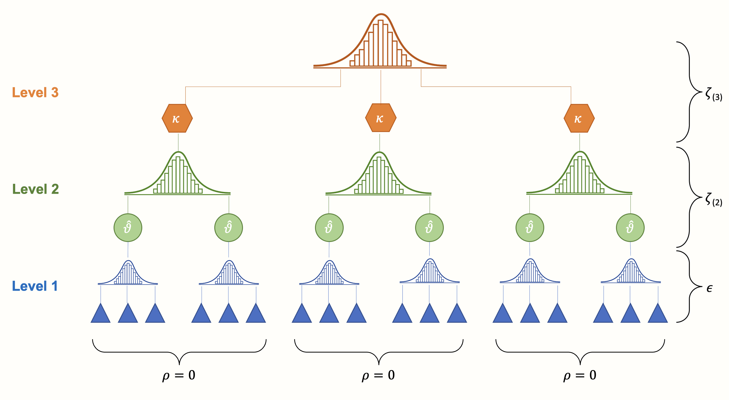
Figure 10.2: In its original form, the three-level (hierarchical) model assumes that effect size estimates within studies or clusters are independent.
In this section, we will therefore devote some time to an extended three-level architecture, the so-called Correlated and Hierarchical Effects (CHE) model (J. E. Pustejovsky and Tipton 2021). Like our previous (hierarchical) three-level model, the CHE model allows to combine several effect sizes into larger clusters, based on certain commonalities (e.g. because they stem from the same study, work group, cultural region, etc.).
But in addition, this model also explicitly takes into account that some effect sizes within clusters are based on the same sample (e.g. because several measurements were taken), and that their sampling errors are therefore correlated. In many real-life scenarios, the CHE model should therefore provide a good starting point; especially when the dependence structure in our data is complex, or only partially known (J. E. Pustejovsky and Tipton 2021)51.
Along with the CHE model, we will also discuss Robust Variance Estimation (RVE) in meta-analytic contexts (L. Hedges, Tipton, and Johnson 2010; Tipton and Pustejovsky 2015; Tipton 2015). This is a set of methods which has been frequently used to handle dependent effect sizes in meta-analyses in the past. In its core, RVE revolves around the so-called Sandwich estimator. This estimator can be used in combination with the CHE model (as well as other meta-analytic models) to obtain robust confidence intervals and \(p\)-values; even when our selected model does not capture the intricate dependence structure of our data perfectly well.
Thus, before fitting our first CHE model, let us start with an overview of meta-analytic RVE as well as the Sandwich estimator, and explore why the latter bears such an appetizing name.
10.4.1 The Sandwich-Type Variance Estimator
In published meta-analyses, the term “robust variance estimation” is sometimes used in a peculiar way, which may lead one to believe that this is a specific method only applicable for meta-analytic data with dependent effect sizes. The opposite is true. The robust variance estimator has originally been developed as a method for conventional regression models, where it is used to calculate the variance of regression weights \(\hat\beta\) (see e.g. Aronow and Miller 2019, chap. 4.2.2).
It is called a “robust” estimator because it provides a consistent estimate of the asymptotic standard error(s); even when usual assumptions of linear models are not met52. Robust estimates of the coefficient variance in a regression model are crucial. The variance estimate53 is used to calculate confidence intervals around the estimated regression weight, as well as \(p\)-values, and thus has direct implications on the inferences we draw from a model.
The type of robust variance estimator we cover here is simply a special version of the original method used in “normal” regression models. Hedges, Tipton and Jackson (2010) laid out an adapted type of RVE that can be used for meta-regression models with dependent effect sizes, and this approach has been extended in the last years few years.
To understand it, we first have to look at the formula of a meta-regression again. Conceptually, this formula is very similar to equation 8.2 presented in Chapter 8.1. We simply display it differently using matrix notation54:
\[\begin{equation} \boldsymbol{T}_{j}=\boldsymbol{X}_{j}\boldsymbol{\beta} + \boldsymbol{u}_j +\boldsymbol{e}_j \tag{10.9} \end{equation}\]
This formula simply tells us that some effect sizes in \(\boldsymbol{T}\) are predicted by regression weights \(\beta\) associated with certain covariates in \(\boldsymbol{X}\). It also tells us that, besides the sampling error (symbolized by \(\boldsymbol{e}_j\)), there are random effects for each study (denoted by \(\boldsymbol{u}_j\)), thus producing a (mixed-effects) meta-regression model.
The special thing are the subscript \(j\)’s in our formula. They, along with the letters in our formula being bold, symbolize that each study or cluster \(j\) in our data set provides, or can provide, more than one effect size. Say that \(n_j\) is the number of effect sizes in some study \(j\). The effect sizes in \(j\) can then be written down as the column vector we see in the formula: \(\boldsymbol{T}_j = (T_{j,1}, \dots, T_{j,{n_j}})^\top\). Similarly, \(\boldsymbol{X}_j\) is the design matrix containing the covariate values of some study \(j\):
\[\begin{equation} \boldsymbol{X}_j = \begin{bmatrix} x_{1,1} & \cdots & x_{1,p} \\ \vdots & \ddots & \vdots \\ x_{n_j,1} & \cdots & x_{n_j,p} \end{bmatrix} \tag{10.10} \end{equation}\]
Where \(p-1\) is the total number of covariates55. The vector of regression coefficients \(\boldsymbol{\beta} = (\beta_1, \dots, \beta_{p})^\top\) we want to estimate contains no subscript \(j\), since it is assumed to be fixed across all studies.
Overall, this notation emphasizes that, when studies can contribute more than one effect size, our data looks like several smaller data sets stacked on top of each other, where \(J\) is the total number of studies or clusters in our data:
\[\begin{equation} \begin{bmatrix} \boldsymbol{T}_1 \\ \boldsymbol{T}_2 \\ \vdots \\ \boldsymbol{T}_J \end{bmatrix} = \begin{bmatrix} \boldsymbol{X}_1 \\ \boldsymbol{X}_2 \\ \vdots \\ \boldsymbol{X}_J \end{bmatrix} \boldsymbol{\beta} + \begin{bmatrix} \boldsymbol{u}_1 \\ \boldsymbol{u}_2 \\ \vdots \\ \boldsymbol{u}_J \end{bmatrix} + \begin{bmatrix} \boldsymbol{e}_1 \\ \boldsymbol{e}_2 \\ \vdots \\ \boldsymbol{e}_J \end{bmatrix}. \tag{10.11} \end{equation}\]
Based on this formula, we can estimate the meta-regression coefficients \(\boldsymbol{\hat\beta}\). To calculate confidence intervals and conduct significance tests of the coefficients, we need an estimate of their variance \(\boldsymbol{V_{\hat\beta}}\). This can be achieved using the robust sampling variance estimator. Its formula looks like this (L. Hedges, Tipton, and Johnson 2010; J. E. Pustejovsky and Tipton 2021, suppl. S1):
\[\begin{equation} \scriptsize\boldsymbol{V}^{\text{R}}_{\boldsymbol{\hat\beta}} = \left(\sum^J_{j=1}\boldsymbol{X}_j^\top\boldsymbol{W}_j\boldsymbol{X}_j \right)^{-1} \left(\sum^J_{j=1}\boldsymbol{X}_j^\top\boldsymbol{W}_j \boldsymbol{A}_j\Phi_j \boldsymbol{A}_j \boldsymbol{W}_j \boldsymbol{X}_j \right) \left(\sum^J_{j=1}\boldsymbol{X}_j^\top\boldsymbol{W}_j\boldsymbol{X}_j \right)^{-1} \tag{10.12} \end{equation}\]
This equation looks quite complicated, and its not necessary to understand every detail. What matters for now is the form and some of the “ingredients” of it.
First, we see that the formula has a tripartite structure. The bracketed components to the left and right are identical, surrounding the part in the middle. This looks like a sandwich, where the outer parts are the “bread” and the inner part is the “meat”, and is the reason for the name “Sandwich estimator”. The crucial “ingredients” of the formula are the \(\boldsymbol{\Phi}_j\), \(\boldsymbol{W}_j\) and \(\boldsymbol{A}_j\) matrices:
The first one, \(\boldsymbol{\Phi}_j=\text{Var}(\boldsymbol{u}_j +\boldsymbol{e}_j)\), is a variance-covariance matrix with \(n_j\) rows and \(n_j\) columns. This matrix describes the true dependence structure of the effect sizes in some study \(j\) (J. E. Pustejovsky and Tipton 2021, Suppl. S1). Unfortunately, it is rarely known how and to what extent effect sizes are correlated within a study; and it is even more difficult to know this for all studies in our meta-analysis. Therefore, it is necessary to make a few simplifying assumptions in our model56. The CHE model, for example, assumes the there is a known correlation \(\rho\) between effect sizes in the same study; and that \(\rho\) has the same value within and across all studies in our meta-analysis (the “constant sampling correlation” assumption, J. E. Pustejovsky and Tipton 2021).
The \(\boldsymbol{W}_j\) matrix contains the weights of each effect size. In previous chapters (see 4.1.1 and 8.1.3), we already learned that we need to take the precision of effect size estimates into account before we can pool them. The optimal way to do this is to take the inverse of the variance, which would mean that \(\boldsymbol{W}_j = \boldsymbol{\Phi}^{-1}_j\). As we mentioned, the true values of \(\boldsymbol{\Phi}_j\) are hardly ever known, so an estimate based on our model, \((\boldsymbol{\hat\Phi}_j)^{-1}\), is used57.
The last part, \(\boldsymbol{A}_j\), is an adjustment matrix, and ensures that the estimator provides valid results even when the number of studies in our meta-analysis is small (say 40 or less, L. Hedges, Tipton, and Johnson 2010; Tipton and Pustejovsky 2015). The recommended approach is to use a matrix based on the bias-reduced linearization, or “CR2” method (Tipton and Pustejovsky 2015)58.
10.4.2 Fitting a CHE Model With Robust Variance Estimation
It is now time to fit our first correlated and hierarchical effects model with R, while employing robust variance estimation to guard our model against misspecification. Like before, we can use the rma.mv function in {metafor} to run our model. This time, we also need some additional functions provided by the {clubSandwich} package (J. Pustejovsky 2022). Therefore, make sure to install the package, and then load it from your library.
As mentioned above, the CHE model assumes that effect sizes within studies or clusters are correlated; and that this correlation is identical within and across studies.
Thus, we have to define a correlation coefficient to be used within our model. For our Chernobyl data, let us assume that the correlation is large, so that \(\rho\)=0.6. This is no more than a guess, and it is highly recommended to run several sensitivity analyses for varying values of \(\rho\).
# constant sampling correlation assumption
rho <- 0.6
Now, using this correlation, we can calculate an assumed variance-covariance matrix for each of our studies. We do this using the impute_covariance_matrix function in {clubSandwich}:
- For the
viargument, we specify the name of the variable in our data set that contains the variance of each effect size (i.e., the squared standard error). - The
clusterargument defines the variable associating each effect size with a study or cluster. In theChernobyldataset, this isauthor. - The
rargument takes the constant correlation coefficient between effect sizes that we assume.
# constant sampling correlation working model
V <- with(Chernobyl,
          impute_covariance_matrix(vi = var.z,
                                   cluster = author,
                                   r = rho))
Using the prepared variance-covariance matrices in V, we can now fit our rma.mv model. Let us say that we want to analyze the same meta-regression model as in Chapter 10.3, in which radiation was used as a covariate.
The arguments look a little different now: the first argument is a formula object, in which we tell the function that our effect sizes z should be predicted by an intercept (1) and the radiation covariate. The V argument takes our list of variance-covariance matrices that we just created; and the sparse argument can be set to TRUE to speed up our computations.
Only the the random and data arguments stay the same. We save the results under the name che.model.
che.model <- rma.mv(z ~ 1 + radiation,
                    V = V,
                    random = ~ 1 | author/es.id,
                    data = Chernobyl,
                    sparse = TRUE)
To calculate the confidence intervals of our meta-regression coefficients, we can use the conf_int function in {clubSandwich}. We only have to provide the fitted model, and specify the small-sample adjustment to be used under vcov. As recommended, we use the "CR2" adjustment (see Chapter 10.4.1).
conf_int(che.model,
         vcov = "CR2")
## Coef. Estimate SE d.f. Lower 95% CI Upper 95% CI
## intrcpt 0.584 0.578 1.00 -6.76 7.93
## radiationlow -0.190 0.605 1.60 -3.52 3.14
## radiationmedium 0.207 0.603 1.98 -2.41 2.83We see that the point estimates under Estimate are similar to the ones we obtained in Chapter 10.3. The estimated standard errors and confidence intervals, however, are much larger. It is also possible to calculate the \(p\)-values of the regression weights using the coef_test function:
coef_test(che.model,
          vcov = "CR2")
## Coef. Estimate SE t-stat d.f. (Satt) p-val (Satt) Sig.
## intrcpt 0.584 0.578 1.010 1.00 0.497
## radiationlow -0.190 0.605 -0.315 1.60 0.789
## radiationmedium 0.207 0.603 0.344 1.98 0.764 We see that none of the coefficients are significant when robust variance estimation is used59.
Robust Variance Estimation & Model Misspecification
Some readers may wonder why we make such a big fuss about using Robust Variance Estimation for our model. The main reason is that multivariate and multilevel models can easily be misspecified. We already learned that even the CHE model is somewhat crude by assuming that correlations are identical within and across studies. Often, it will be somewhat unclear if our model approximates the complex dependencies in our data reasonably well.
Robust variance estimates are helpful in this respect because they allow to guard our inferences (i.e., the confidence intervals and \(p\)-values we calculate) against potential misspecification of our model.
The {robumeta} package
In this section, we covered robust variance estimation in combination with the correlated and hierarchical effects model. This model, together with a few other innovations, has been proposed by Pustejosky and Tipton (2021).
The “original” RVE approach by Hedges, Tipton and Jackson (2010), along with a few small-sample extensions, can be applied using the {robumeta} package (Z. Fisher, Tipton, and Zhipeng 2017). The package allows to fit a meta-regression using the two model types originally proposed by Hedges, Tipton and Jackson: the hierarchical, as well as the correlated effects model (but not both combined).
10.5 Cluster Wild Bootstrapping
In the last chapter, we learned how to fit a correlated and hierarchical effects model, and how to calculate confidence intervals and coefficient tests using robust variance estimation.
Another, and sometimes favorable way to test coefficients in our model are bootstrapping procedures, a special variant of which is so-called cluster wild bootstrapping (Joshi, Pustejovsky, and Beretvas 2021). This method is well suited if the total number of studies \(J\) in our meta-analysis is small; especially compared to RVE, which can lead to overly conservative results in small samples (as we have seen in our own Chernobyl example).
This method is also sensible whenever we want to test so-called multiple-contrast hypotheses. Multiple-constrast hypotheses are needed, for example, if we want to test the overall effect of a dummy-coded categorical covariate.
The Cluster Wild Bootstrapping Algorithm
The wild bootstrap is a method based on the residuals of a null model (i.e. a model fitted without any additional covariates). In cluster wild bootstrapping, residuals are transformed using an adjustment matrix \(\boldsymbol{A}_j\), for example based on the CR2 method (see Chapter 10.4.1), to handle dependent effect sizes. A general algorithm for wild boostrapping looks like this (Joshi, Pustejovsky, and Beretvas 2021):
- Calculate the full model based on the original data, and derive the test statistic of interest (e.g. a \(t\) or \(F\) value).
- Fit a null model based on the original data and extract its residuals \(\boldsymbol{e}\).
- For each study or cluster \(j\), draw a random value from a distribution60; multiply the residuals of \(j\) by this random value.
- Generate new, bootstrapped effect sizes by adding the transformed residuals to the predicted values of the null model based on the original data.
- Fit the full model again, using the bootstrapped effect size values; calculate the test statistic again.
Steps 3 to 5 are then repeated \(R\) times. The boostrap \(p\)-value can be derived as the proportion of times the boostrap test statistic was more extreme than the one based on the original data.
To test multiple-contrast hypotheses using the bootstrap, we can use the {wildmeta} package (Joshi and Pustejovsky 2022). This package needs to be installed and loaded from the library for our next example. Furthermore, using functions of the {tidyverse}, we generate a new variable in our Chernobyl data set, in which we save the year of each study.
# Make sure {wildmeta} and {tidyverse} is loaded
library(wildmeta)
library(tidyverse)

# Add year as extra variable
Chernobyl$year <- str_extract(Chernobyl$author,
                              "[0-9]{4}") %>% as.numeric()
Next, we use this variable as a new predictor in our rma.mv meta-regression model. We simply add year to the formula in the first argument, while applying the scale function to center and scale the covariate. There is also another thing we do in the formula: we change the 1 of the intercept to a 0. This means that there is no intercept, and that predictions of year are stratified by different levels of radiation61. We save the result as che.model.bs.
che.model.bs <- rma.mv(z ~ 0 + radiation + scale(year),
                       V = V,
                       random = ~ 1 | author/es.id,
                       data = Chernobyl,
                       sparse = TRUE)
Before we start bootstrapping, we need to define a linear contrast for the test we want to conduct. Let us say that we want to test the overall moderation effect of our radiation variable. To do this, we have to use the constrain_equal function in {clubSandwich} to create a constraint matrix for out test. The null hypothesis is that effects are equal among all three levels of our radiation variable, so we set the constraints argument to 1:3. Furthermore, we specify the coefs argument by providing the coefficients of the model we just fitted. We save the results as rad.constraints.
rad.constraints <- constrain_equal(constraints = 1:3,
                                   coefs = coef(che.model.bs))
rad.constraints
## [,1] [,2] [,3] [,4]
## [1,] -1 1 0 0
## [2,] -1 0 1 0We can now calculate the bootstrap \(p\)-value of the multiple-contrast hypothesis, using the Wald_test_cwb function in {wildmeta}. We have to specify our fitted full model, our constraint matrix, the type of small-sample adjustment we want to use, as well as R, the number of bootstrap replications. It is recommended to use a high number of replications (e.g. 1000 or more), since this improves our power. In our example, we use 2000 replications, and save the results as cw.boot. Please note that, depending on the number of iterations, this process can take several minutes to finish.
cw.boot <- Wald_test_cwb(full_model = che.model.bs,
                         constraints = rad.constraints,
                         adjust = "CR2",
                         R = 2000)
cw.boot
## Test Adjustment CR_type Statistic R p_val
## 1 CWB Adjusted CR2 CR0 Naive-F 2000 0.3595We see that the \(p\)-value of our test of moderation is 0.36, which is not significant. We had a similar finding in our previous moderator analysis of the radiation strength in Chapter 10.3.
Using the plot function, we can also visualize the density of the test statistics across all bootstrap replications.
plot(cw.boot,
     fill = "lightblue",
     alpha = 0.5)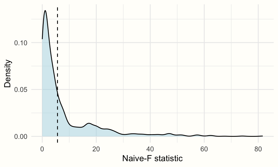
10.6 Questions & Answers
Test your knowledge!
- Why is it more accurate to speak of “three-level” instead of “multilevel” models?
- When are three-level meta-analysis models useful?
- Name two common causes of effect size dependency.
- How can the multilevel \(I^2\) statistic be interpreted?
- How can a three-level model be expanded to incorporate the effect of moderator variables?
Answers to these questions are listed in Appendix A at the end of this book.
\[\tag*{$\blacksquare$}\]
10.7 Summary
All random-effects meta-analyses are based on a multilevel model. When a third layer is added, we speak of a three-level meta-analysis model. Such models are well suited to handle clustered effect size data.
Three-level models can be used for dependent effect sizes. When a study contributes more than one effect size, for example, we typically can not assume that these results are independent. Three-level model control for this problem by assuming that effect sizes are nested in larger clusters (e.g. studies).
In contrast to a conventional meta-analysis, three-level models estimate two heterogeneity variances: the random-effects variance within clusters, and the between-cluster heterogeneity variance.
It is also possible to test categorical or continuous predictors using a three-level model. This results in a three-level mixed-effects model.