Chapter 11 Regression
11.1 Introduction to Regression
Regression is a fundamental statistical and machine-learning technique used to model the relationship between a dependent variable (response) and one or more independent variables (predictors). The primary goal of regression is to understand how changes in predictors affect the response variable, make predictions, and identify significant relationships.
Regression analysis is used in various domains, including biology, economics, engineering, and social sciences. For example, researchers may use regression to predict flower petal lengths (dependent variable) based on sepal widths (independent variable) in the famous Iris dataset.
Key Concepts in Regression
Dependent Variable: The outcome or response variable.
Independent Variables: The predictors or explanatory variables.
11.2 Types of Regression
This section introduces popular regression techniques with examples from the Iris dataset. Each regression type includes code for fitting the model and customized visualizations using R’s plotting libraries.
11.2.1 Simple Linear Regression
Models the relationship between one dependent and one independent variable.
# Load data
data(iris)

# Fit linear model
lm_model <- lm(Petal.Length ~ Sepal.Length, data = iris)

# Print summary
summary(lm_model)
##
## Call:
## lm(formula = Petal.Length ~ Sepal.Length, data = iris)
##
## Residuals:
## Min 1Q Median 3Q Max
## -2.47747 -0.59072 -0.00668 0.60484 2.49512
##
## Coefficients:
## Estimate Std. Error t value Pr(>|t|)
## (Intercept) -7.10144 0.50666 -14.02 <2e-16 ***
## Sepal.Length 1.85843 0.08586 21.65 <2e-16 ***
## ---
## Signif. codes: 0 '***' 0.001 '**' 0.01 '*' 0.05 '.' 0.1 ' ' 1
##
## Residual standard error: 0.8678 on 148 degrees of freedom
## Multiple R-squared: 0.76, Adjusted R-squared: 0.7583
## F-statistic: 468.6 on 1 and 148 DF, p-value: < 2.2e-16library(ggplot2)
# Custom visualization settings
ggplot(iris, aes(x = Sepal.Length, y = Petal.Length)) +
geom_point(color = "steelblue") +
geom_smooth(method = "lm", se = FALSE, color = "darkred") +
ggtitle("Simple Linear Regression: Sepal Length vs Petal Length") +
xlab("Sepal Length (cm)") +
ylab("Petal Length (cm)") +
theme_minimal(base_size = 14) +
theme(plot.title = element_text(size = 16, hjust = 0.5, color = "darkblue")) 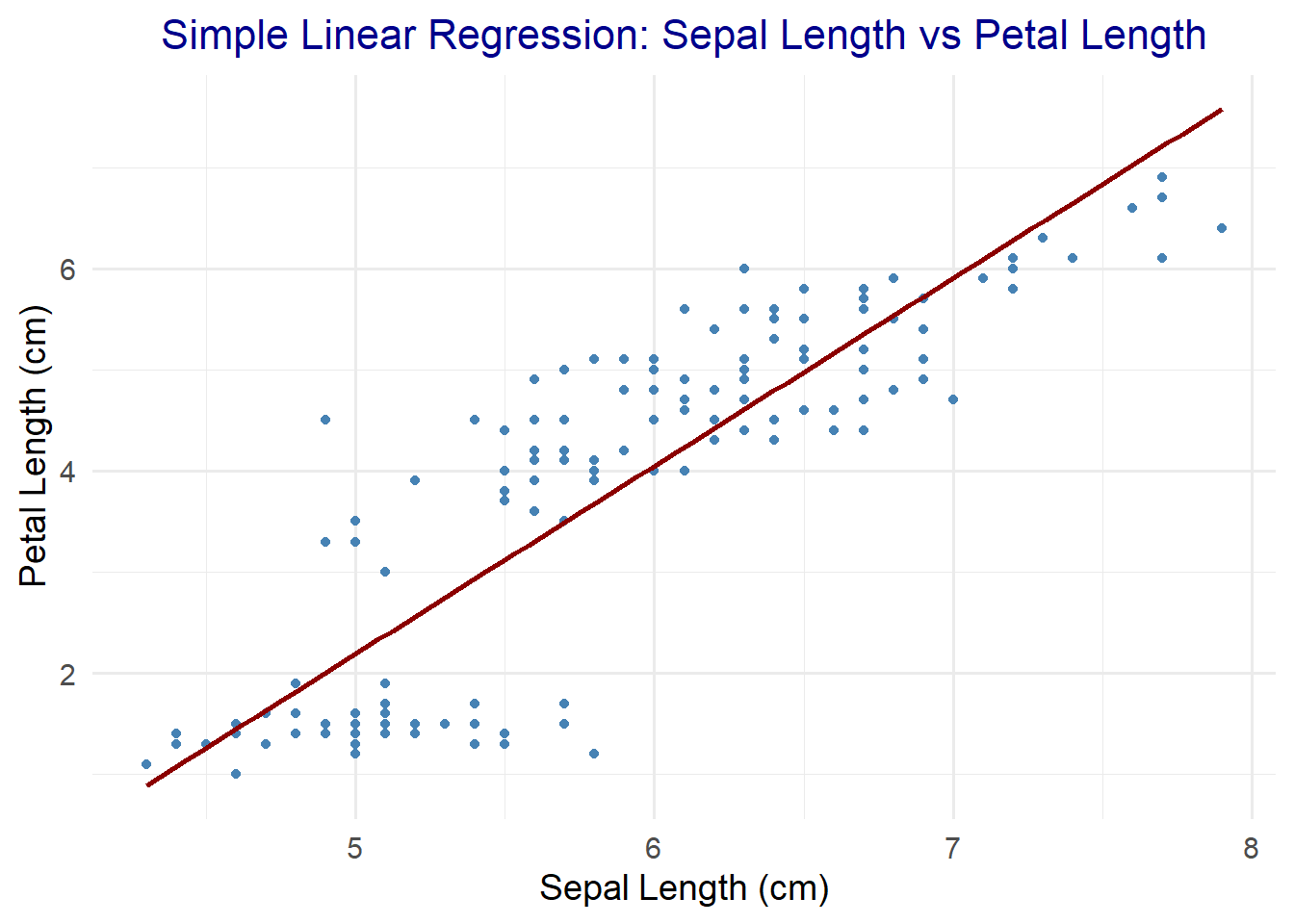
11.2.2 Multiple Linear Regression
Examines the relationship between a dependent variable and multiple independent variables.
# Fit multiple linear regression model
multi_lm_model <- lm(Petal.Length ~ Sepal.Length + Sepal.Width, data = iris)

# Print summary
summary(multi_lm_model)
##
## Call:
## lm(formula = Petal.Length ~ Sepal.Length + Sepal.Width, data = iris)
##
## Residuals:
## Min 1Q Median 3Q Max
## -1.25582 -0.46922 -0.05741 0.45530 1.75599
##
## Coefficients:
## Estimate Std. Error t value Pr(>|t|)
## (Intercept) -2.52476 0.56344 -4.481 1.48e-05 ***
## Sepal.Length 1.77559 0.06441 27.569 < 2e-16 ***
## Sepal.Width -1.33862 0.12236 -10.940 < 2e-16 ***
## ---
## Signif. codes: 0 '***' 0.001 '**' 0.01 '*' 0.05 '.' 0.1 ' ' 1
##
## Residual standard error: 0.6465 on 147 degrees of freedom
## Multiple R-squared: 0.8677, Adjusted R-squared: 0.8659
## F-statistic: 482 on 2 and 147 DF, p-value: < 2.2e-16Create a scatter plot matrix for a broader view of relationships.
library(GGally)

# Scatter plot matrix
ggpairs(iris, columns = 1:4, aes(color = Species)) +
  ggtitle("Scatter Plot Matrix for Iris Dataset") +
theme(plot.title = element_text(size = 16, hjust = 0.5, color = "darkgreen")) 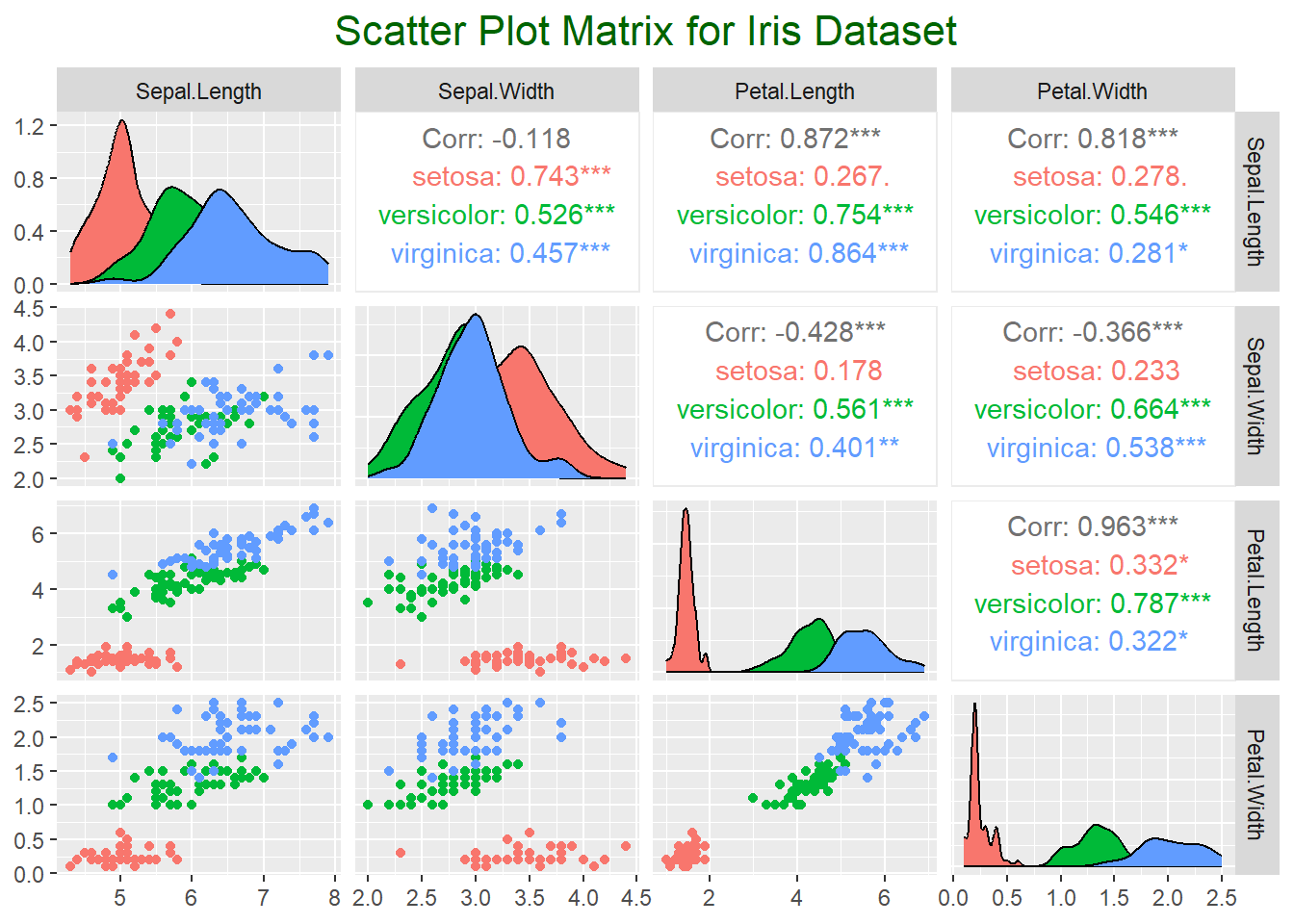
11.2.3 Polynomial Regression
Extends linear regression to model non-linear relationships.
# Fit polynomial model
poly_model <- lm(Petal.Length ~ poly(Sepal.Length, 2), data = iris)

# Print summary
summary(poly_model)
##
## Call:
## lm(formula = Petal.Length ~ poly(Sepal.Length, 2), data = iris)
##
## Residuals:
## Min 1Q Median 3Q Max
## -2.6751 -0.5138 0.1218 0.5356 2.6287
##
## Coefficients:
## Estimate Std. Error t value Pr(>|t|)
## (Intercept) 3.75800 0.06847 54.888 < 2e-16 ***
## poly(Sepal.Length, 2)1 18.78473 0.83854 22.402 < 2e-16 ***
## poly(Sepal.Length, 2)2 -2.84550 0.83854 -3.393 0.000887 ***
## ---
## Signif. codes: 0 '***' 0.001 '**' 0.01 '*' 0.05 '.' 0.1 ' ' 1
##
## Residual standard error: 0.8385 on 147 degrees of freedom
## Multiple R-squared: 0.7774, Adjusted R-squared: 0.7744
## F-statistic: 256.7 on 2 and 147 DF, p-value: < 2.2e-16ggplot(iris, aes(x = Sepal.Length, y = Petal.Length)) +
geom_point(color = "steelblue") +
geom_smooth(method = "lm", formula = y ~ poly(x, 2), se = FALSE, color = "darkorange") +
ggtitle("Polynomial Regression: Sepal Length vs Petal Length") +
xlab("Sepal Length (cm)") +
ylab("Petal Length (cm)") +
theme_minimal(base_size = 14) +
theme(plot.title = element_text(size = 16, hjust = 0.5, color = "darkorange")) 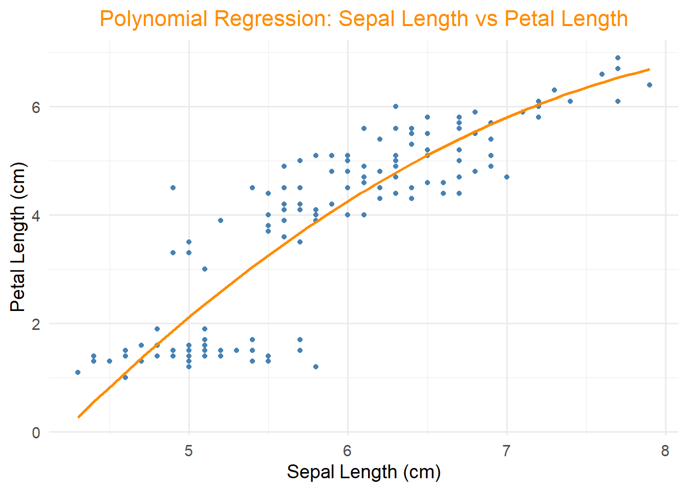
Used when the dependent variable is categorical.
# Fit logistic regression model
logistic_model <- glm(Species ~ Petal.Length + Petal.Width, data = iris, family = "binomial")

# Print summary
summary(logistic_model)
##
## Call:
## glm(formula = Species ~ Petal.Length + Petal.Width, family = "binomial",
## data = iris)
##
## Deviance Residuals:
## Min 1Q Median 3Q Max
## -3.970e-05 -2.100e-08 2.100e-08 2.100e-08 4.718e-05
##
## Coefficients:
## Estimate Std. Error z value Pr(>|z|)
## (Intercept) -69.45 43042.94 -0.002 0.999
## Petal.Length 17.60 43449.07 0.000 1.000
## Petal.Width 33.89 115850.84 0.000 1.000
##
## (Dispersion parameter for binomial family taken to be 1)
##
## Null deviance: 1.9095e+02 on 149 degrees of freedom
## Residual deviance: 5.1700e-09 on 147 degrees of freedom
## AIC: 6
##
## Number of Fisher Scoring iterations: 25library(ggplot2)
ggplot(iris, aes(x = Petal.Length, y = Petal.Width, color = Species)) +
geom_point(size = 3) +
ggtitle("Logistic Regression: Decision Boundary") +
xlab("Petal Length (cm)") +
ylab("Petal Width (cm)") +
theme_minimal(base_size = 14) +
theme(plot.title = element_text(size = 16, hjust = 0.5, color = "purple")) 
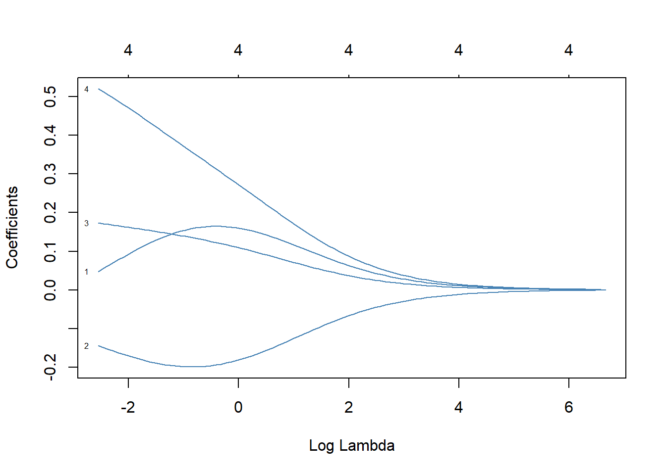
11.2.4 Ridge and Lasso Regression
Used to handle multicollinearity and feature selection in datasets with many predictors.
Example: Regularized regression with glmnet
library(glmnet)

# Prepare data
x <- as.matrix(iris[, 1:4])
y <- as.numeric(iris$Species)

# Fit ridge regression
ridge_model <- glmnet(x, y, alpha = 0)

# Fit lasso regression
lasso_model <- glmnet(x, y, alpha = 1)
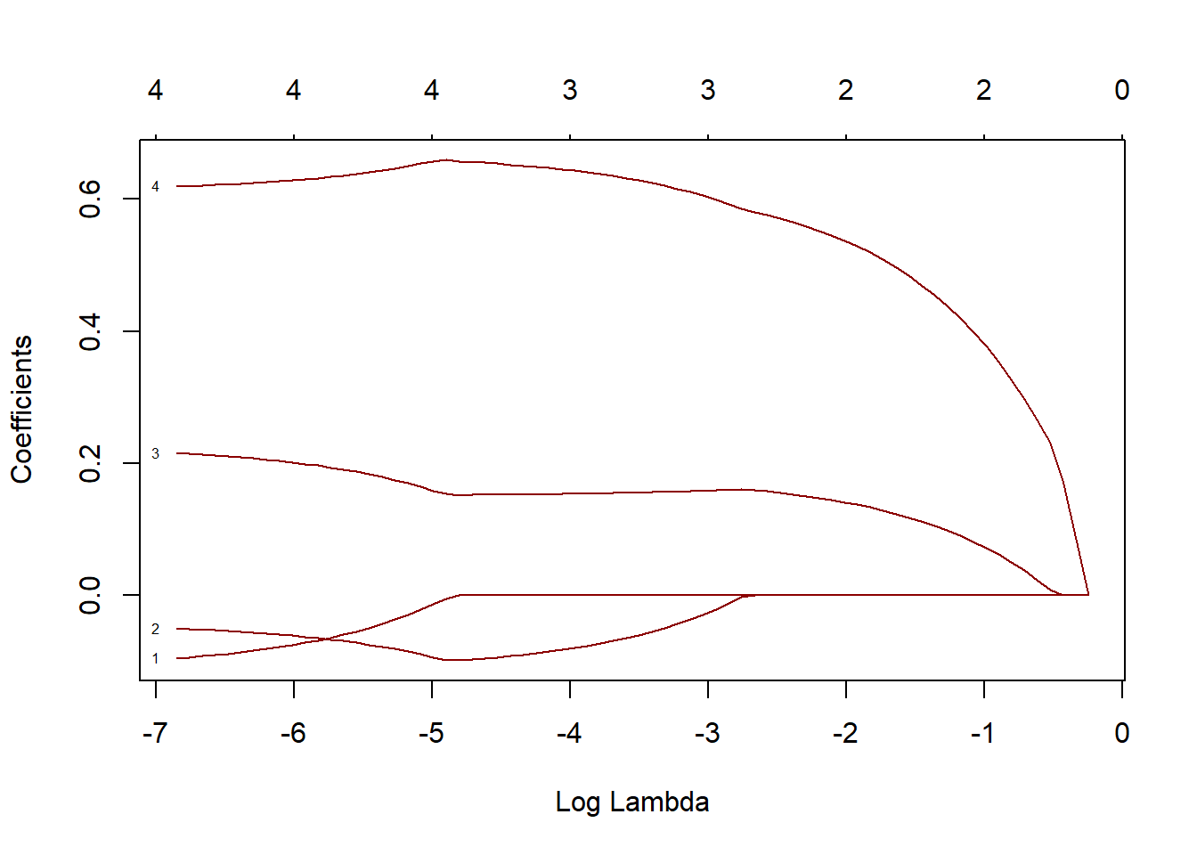
Plot the coefficient paths for ridge and lasso regression.
11.3 Summary
In this chapter, we explored various regression techniques, from simple linear models to more advanced methods like logistic, ridge, and lasso regression, using the Iris dataset as an example. Custom visualizations were created for each method, emphasizing clear, publication-quality designs with tailored aesthetics. Understanding these regression techniques equips analysts with the tools to model and interpret complex relationships in real-world datasets.