Chapter 13 Classification
13.1 Introduction
Classification is a core technique in machine learning, enabling the prediction of categories or labels for a given dataset. In food science, classification applications range from identifying food quality grades to determining ingredient origins and even classifying food types based on sensory attributes.
This chapter introduces classification using the Iris dataset, a well-known dataset that serves as an excellent educational tool for understanding the fundamentals of machine learning. We will demonstrate four classification models: Random Forests, and Support Vector Machines (SVM). By the end of this chapter, you will have practical knowledge of implementing, visualizing, and evaluating classification models in R.
13.2 Setting Up the Environment
Ensure you have the necessary libraries installed:
Load the required libraries:
13.3 Data Preparation
We start by loading and preparing the Iris dataset for analysis. The dataset contains measurements of sepal and petal characteristics for three flower species: setosa, versicolor, and virginica.
##   Sepal.Length Sepal.Width Petal.Length Petal.Width Species
## 1          5.1         3.5          1.4         0.2  setosa
## 2          4.9         3.0          1.4         0.2  setosa
## 3          4.7         3.2          1.3         0.2  setosa
## 4          4.6         3.1          1.5         0.2  setosa
## 5          5.0         3.6          1.4         0.2  setosa
## 6 5.4 3.9 1.7 0.4 setosa13.4 Decision Tree
Decision Trees classify data by iteratively splitting it based on feature thresholds.
# Train a Decision Tree model
tree_model <- rpart(Species ~ ., data = train_data, method = "class")

# Visualize the Decision Tree
rpart.plot(tree_model, type = 3, extra = 102)
# Predict on the test set
tree_predictions <- predict(tree_model, test_data, type = "class")

# Evaluate performance
tree_conf_matrix <- confusionMatrix(tree_predictions, test_data$Species)
print(tree_conf_matrix)
## Confusion Matrix and Statistics
##
## Reference
## Prediction setosa versicolor virginica
## setosa 15 0 0
## versicolor 0 14 2
## virginica 0 1 13
##
## Overall Statistics
##
## Accuracy : 0.9333
## 95% CI : (0.8173, 0.986)
## No Information Rate : 0.3333
## P-Value [Acc > NIR] : < 2.2e-16
##
## Kappa : 0.9
##
## Mcnemar's Test P-Value : NA
##
## Statistics by Class:
##
## Class: setosa Class: versicolor Class: virginica
## Sensitivity 1.0000 0.9333 0.8667
## Specificity 1.0000 0.9333 0.9667
## Pos Pred Value 1.0000 0.8750 0.9286
## Neg Pred Value 1.0000 0.9655 0.9355
## Prevalence 0.3333 0.3333 0.3333
## Detection Rate 0.3333 0.3111 0.2889
## Detection Prevalence 0.3333 0.3556 0.3111
## Balanced Accuracy 1.0000 0.9333 0.916713.5 Random Forest
Random Forests combine multiple decision trees to improve accuracy and reduce overfitting.
# Train a Random Forest model
rf_model <- randomForest(Species ~ ., data = train_data, ntree = 100)

# Predict on the test set
rf_predictions <- predict(rf_model, test_data)

# Evaluate performance
rf_conf_matrix <- confusionMatrix(rf_predictions, test_data$Species)
print(rf_conf_matrix)
## Confusion Matrix and Statistics
##
## Reference
## Prediction setosa versicolor virginica
## setosa 15 0 0
## versicolor 0 14 2
## virginica 0 1 13
##
## Overall Statistics
##
## Accuracy : 0.9333
## 95% CI : (0.8173, 0.986)
## No Information Rate : 0.3333
## P-Value [Acc > NIR] : < 2.2e-16
##
## Kappa : 0.9
##
## Mcnemar's Test P-Value : NA
##
## Statistics by Class:
##
## Class: setosa Class: versicolor Class: virginica
## Sensitivity 1.0000 0.9333 0.8667
## Specificity 1.0000 0.9333 0.9667
## Pos Pred Value 1.0000 0.8750 0.9286
## Neg Pred Value 1.0000 0.9655 0.9355
## Prevalence 0.3333 0.3333 0.3333
## Detection Rate 0.3333 0.3111 0.2889
## Detection Prevalence 0.3333 0.3556 0.3111
## Balanced Accuracy 1.0000 0.9333 0.916713.6 Support Vector Machine (SVM)
SVM finds the hyperplane that best separates the classes. It can also handle non-linear data using kernel functions.
# Train an SVM model
svm_model <- svm(Species ~ ., data = train_data, kernel = "radial")

# Predict on the test set
svm_predictions <- predict(svm_model, test_data)

# Evaluate performance
svm_conf_matrix <- confusionMatrix(svm_predictions, test_data$Species)
print(svm_conf_matrix)
## Confusion Matrix and Statistics
##
## Reference
## Prediction setosa versicolor virginica
## setosa 15 0 0
## versicolor 0 14 2
## virginica 0 1 13
##
## Overall Statistics
##
## Accuracy : 0.9333
## 95% CI : (0.8173, 0.986)
## No Information Rate : 0.3333
## P-Value [Acc > NIR] : < 2.2e-16
##
## Kappa : 0.9
##
## Mcnemar's Test P-Value : NA
##
## Statistics by Class:
##
## Class: setosa Class: versicolor Class: virginica
## Sensitivity 1.0000 0.9333 0.8667
## Specificity 1.0000 0.9333 0.9667
## Pos Pred Value 1.0000 0.8750 0.9286
## Neg Pred Value 1.0000 0.9655 0.9355
## Prevalence 0.3333 0.3333 0.3333
## Detection Rate 0.3333 0.3111 0.2889
## Detection Prevalence 0.3333 0.3556 0.3111
## Balanced Accuracy 1.0000 0.9333 0.916713.7 Model Comparison
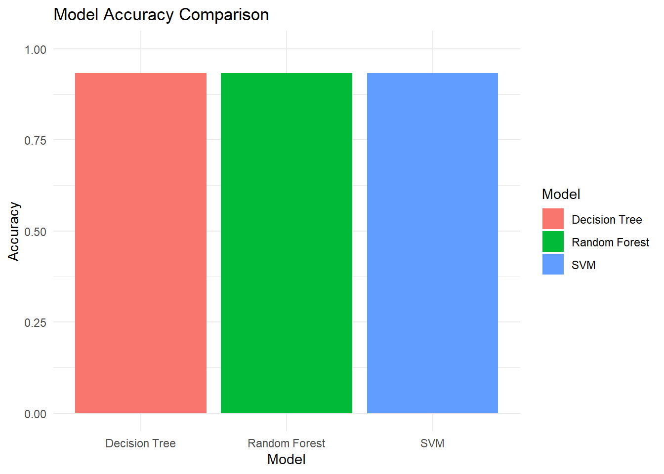
We compare the accuracy of the four models to identify their strengths and weaknesses.
# Compile model accuracies
results <- data.frame(
  Model = c("Decision Tree", "Random Forest", "SVM"),
  Accuracy = c(
    tree_conf_matrix$overall["Accuracy"],
    rf_conf_matrix$overall["Accuracy"],
    svm_conf_matrix$overall["Accuracy"]
  )
)

# Visualize the comparison
ggplot(results, aes(x = Model, y = Accuracy, fill = Model)) +
  geom_bar(stat = "identity") +
  ylim(0, 1) +
  labs(
    title = "Model Accuracy Comparison",
    y = "Accuracy",
    x = "Model"
  ) +
  theme_minimal()
13.8 Summary
Each classification model offers unique advantages:
Decision Trees: Highly interpretable but prone to overfitting on complex datasets.
Random Forests: Robust and accurate, ideal for complex, noisy data, but less interpretable.
SVM: Excellent for non-linear data, but computationally intensive for large datasets.