Chapter 7 Normality
7.2 Introduction to Normality
Normality refers to whether a dataset or variable follows a normal distribution, also known as the Gaussian distribution. This distribution is characterized by its symmetric bell-shaped curve, where most of the data points cluster around the mean, and the probabilities taper off equally on both sides. Many statistical tests and models, such as ANOVA, t-tests, and linear regression, assume that the data is normally distributed, making normality a critical concept in data analysis.
7.2.1 Key Characteristics of a Normal Distribution
Symmetry: The curve is symmetric about the mean.
Mean = Median = Mode: All three central tendency measures are the same.
Empirical Rule:
68% of data falls within 1 standard deviation of the mean.
95% of data falls within 2 standard deviations.
99.7% of data falls within 3 standard deviations.
7.2.2 Why Normality Matters
- Statistical Assumptions: Many parametric tests rely on the assumption of normality.
- Model Performance: Non-normal data can distort parameter estimation and reduce model accuracy.
- Error Analysis: Residuals (errors) in regression analysis should ideally follow a normal distribution.
7.3 Normality detection
The data of most food experiments will be analyzed for significance. In the method section of many articles, we will mention what method is used for significance analysis. If P is less than 0.05, the difference between variables is considered to be significant. However, before the significance analysis, some preprocessing shoule carried out to make sure Normal distribution, otherwise the result is inaccurate. The following summarizes the data preprocessing that can be performed in R to meet the requirements of saliency analysis.
Before statistical analysis of data such as significance analysis, the data should meet normally distributed.
##
##  Shapiro-Wilk normality test
##
## data:  Apple
## W = 0.94874, p-value = 0.7301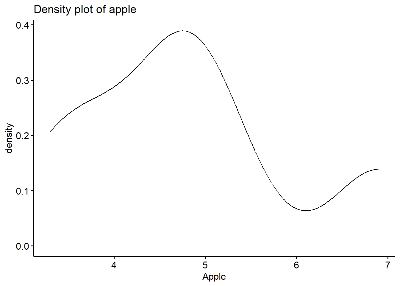
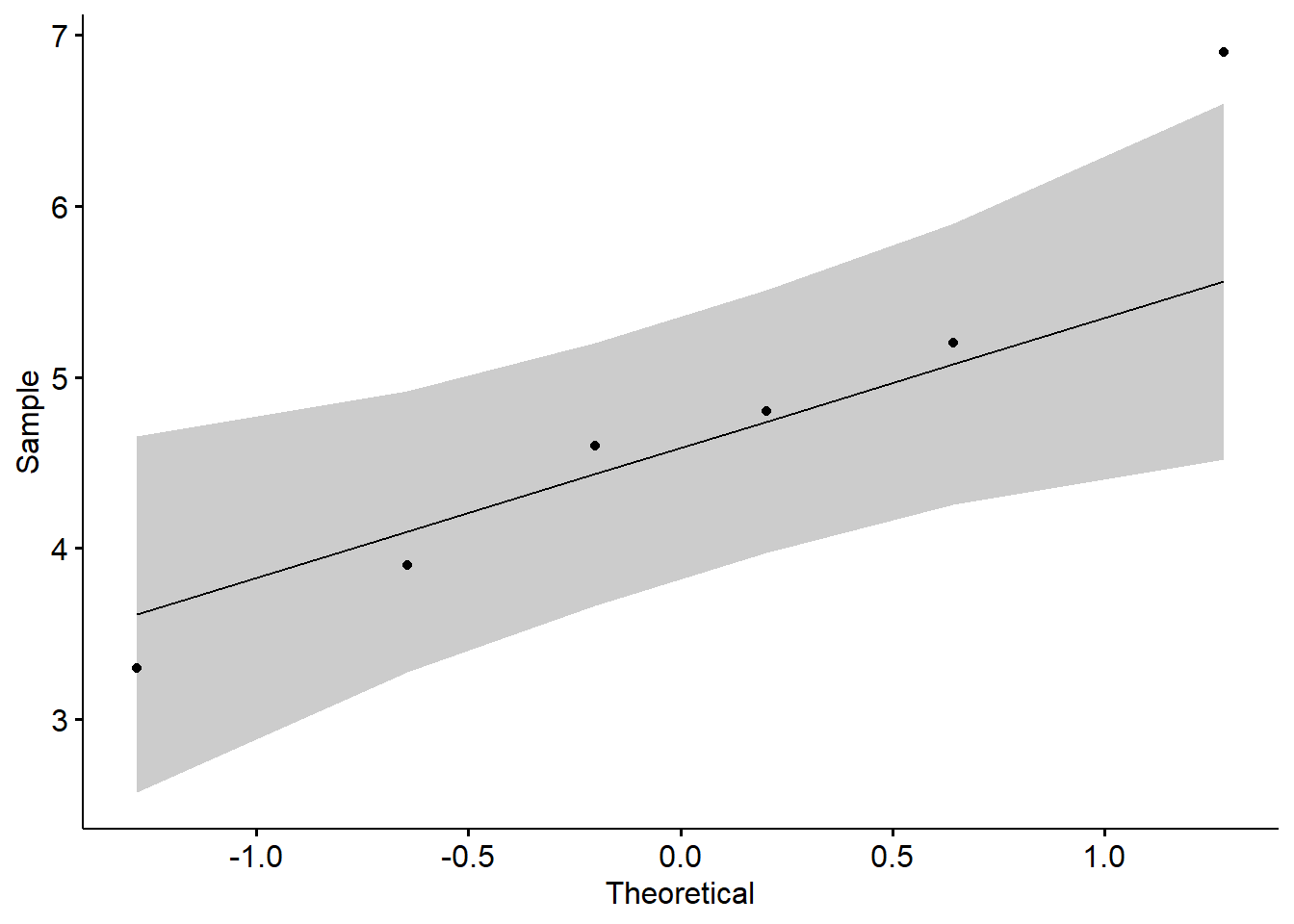
Shapiro-Wilk normality test
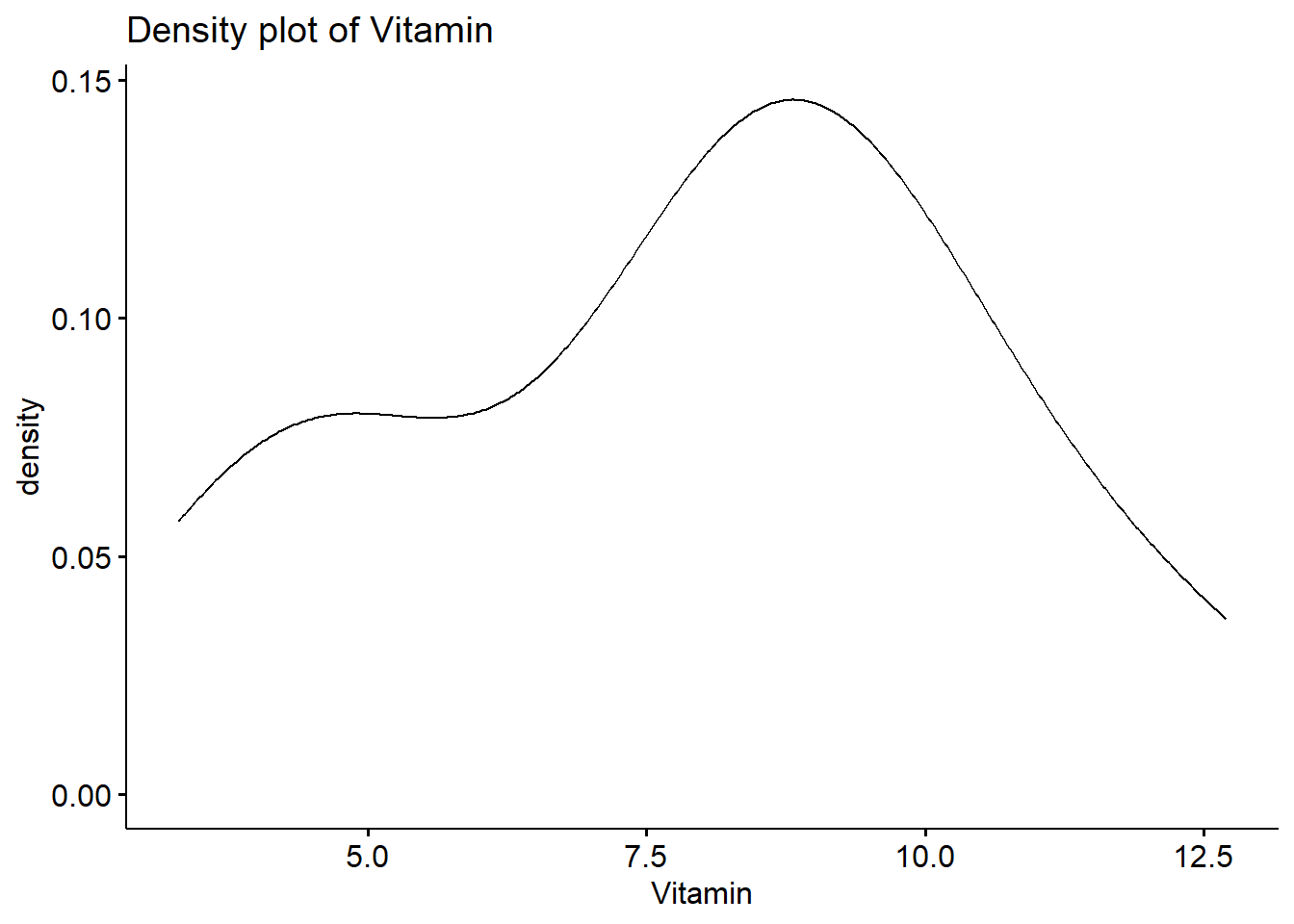
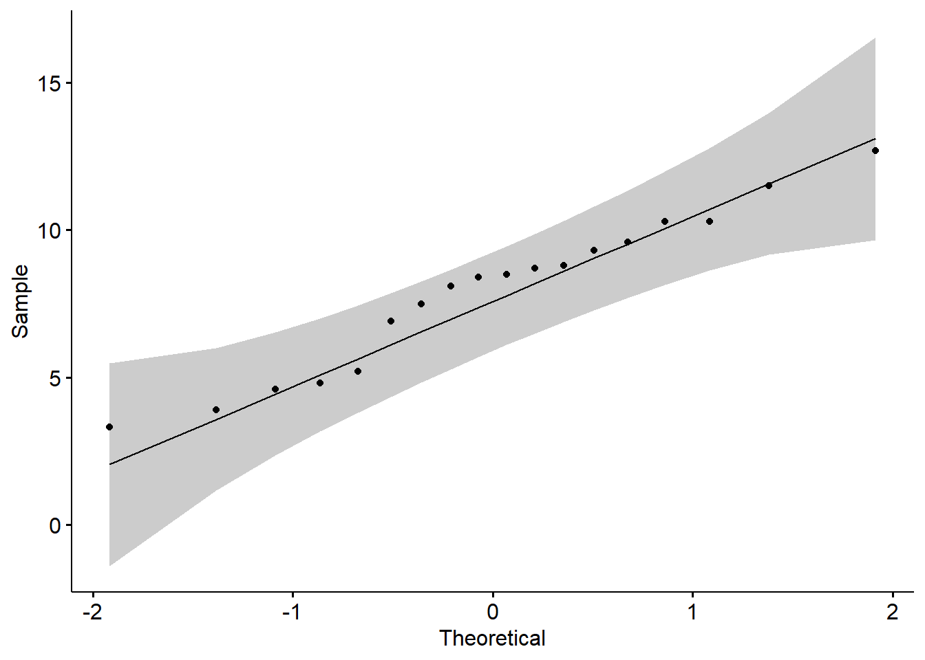
data: data$Vitamin W = 0.96026, p-value = 0.6066 When the P value here is greater than 0.05, it represents a normal distribution.
You can also observe the normal distribution graph:
7.4 Defination of ANOVA
Analysis of variance (ANOVA) is an analysis tool used in statistics that splits an observed aggregate variability found inside a data set into two parts: systematic factors and random factors. The systematic factors have a statistical influence on the given data set, while the random factors do not. Analysts use the ANOVA test to determine the influence that independent variables have on the dependent variable in a regression study– cited from WILL KENTON(https://www.investopedia.com/terms/a/anova.asp)
7.5 The examples of ANOVA using fruit dataset
library(multcomp)
library(dplyr)
setwd("C:/local_R/Dataset")
data <- read.csv("fruits_Vc.csv")
head(data)
## Number Fruit Repeat Vitamin
## 1 1 Apple A1 4.6
## 2 2 Apple A2 3.9
## 3 3 Apple A3 5.2
## 4 4 Apple A4 6.9
## 5 5 Apple A5 4.8
## 6 6 Apple A6 3.3To compare the vitamin C contents of different fruits
data$Fruit = as.factor(data$Fruit)
VitaminC <- data$Vitamin
Fruits <- data$Fruit

aggregate(VitaminC, by =list(Fruits), FUN=mean)
## Group.1 x
## 1 Apple 4.783333
## 2 Banana 10.266667
## 3 Watermelon 8.683333## Group.1 x
## 1 Apple 1.2384130
## 2 Banana 1.5807171
## 3 Watermelon 0.9847165## Df Sum Sq Mean Sq F value Pr(>F)
## Fruits 2 95.57 47.78 28.66 7.52e-06 ***
## Residuals 15 25.01 1.67
## ---
## Signif. codes: 0 '***' 0.001 '**' 0.01 '*' 0.05 '.' 0.1 ' ' 1## Tukey multiple comparisons of means
## 95% family-wise confidence level
##
## Fit: aov(formula = VitaminC ~ Fruits)
##
## $Fruits
## diff lwr upr p adj
## Banana-Apple 5.483333 3.546906 7.4197605 0.0000068
## Watermelon-Apple 3.900000 1.963573 5.8364272 0.0002819
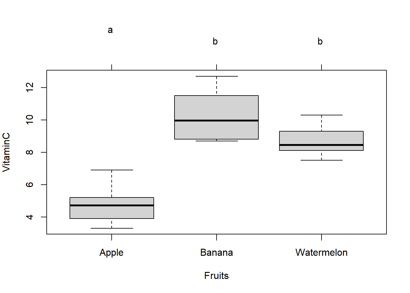
## Watermelon-Banana -1.583333 -3.519761 0.3530938 0.1184352par(mar=c(5,4,6,2))
data$Fruit = as.factor(data$Fruit)
tuk <- glht(fit,linfct= mcp(Fruits="Tukey"))
p1 <- plot(cld(tuk,level=.05),col="lightgrey")