14 Topic modelling
Another text mining tool which can be useful in exploring newspaper data is topic modelling. Topic modelling tried to discern a bunch of ‘topics’, expressed as a set of important keywords, from a group of documents. It works best if each document covers one clear subject. To demonstrate the value to newspaper data, I’ll talk through an example of applying the tutorial as written here: https://www.tidytextmining.com
14.1 Topic modelling with the library ‘topicmodels’
First, load and install the relevant lirbraries. If you’ve loaded the notebooks into Rstudio, it should detect and ask if you want to install any missing ones, but you might need to use install_packages() if not.
library(tidyverse)
library(tidytext)
library(topicmodels)
14.2 Load the tokenised dataframe
Load the tokenised dataframe created in the term_frequency notebook - this is the dataframe with one word per row.
load('tokenised_news_sample')14.3 Create a dataframe of word counts with tf_idf scores
Like in the tf_idf notebook, make a dataframe of the words in each document, with the count and the tf-idf score. This will be used to filter and weight the text data.
First, get the word counts for each article. An optional step would be to filter to include only English-language words and some common nouns.
issue_words = tokenised_news_sample %>%
  filter(word %in% grady_augmented) %>%
  mutate(issue_code = paste0(title, full_date)) %>%
  group_by(issue_code, word) %>%
  tally() %>%
  arrange(desc(n))
Next, use bind_tf_idf() to get the tf_idf scores.
issue_words = issue_words %>% bind_tf_idf(word, issue_code, n)14.4 Make a ‘document term matrix’
Using the function cast_dtm() from the topicmodels package, make a document term matrix. This is a matrix with all the documents on one axis, all the words on the other, and the number of times that word appears as the value. We’ll also filter out words with a low tf-idf score, and only include words that occur at least 5 times.
dtm_long <- issue_words %>%
    filter(tf_idf > 0.00006) %>%
  filter(n>5) %>%
    cast_dtm(issue_code, word, n)
Use the LDA() function to produce the model. You specify the number of topics in advance, using the argument k, and we’ll set the random seed to a set number for reproducibility. The method algorithm used here is known as Latent Dirichlet Allocation - it uses the distribution of words in each document to group them together into ‘topics’. It can take some time to run the model - be prepared to wait a bit.
lda_model_long_1 <- LDA(dtm_long,k = 25, control = list(seed = 1234))There are two things we can do now: first, get a list of words scored by how they contributed to each of the topics.
result <- tidytext::tidy(lda_model_long_1, 'beta')We can plot the top words which make up each of the topics, to get an idea of how the articles have been categorised. Some of these make sense: there’s a topic which seems to be about university and education, one with words relating to poor laws, and a couple about disease in the army, as well as some more which contain words probably related to the Crimean war.
result %>%
    group_by(topic) %>%
    top_n(5, beta) %>%
    ungroup() %>%
    arrange(topic, -beta) %>%
    mutate(term = reorder(term, beta)) %>%
    ggplot(aes(term, beta, fill = factor(topic))) +
    geom_col(show.legend = FALSE) +
    facet_wrap(~ topic, scales = "free", ncol = 4) +
    coord_flip()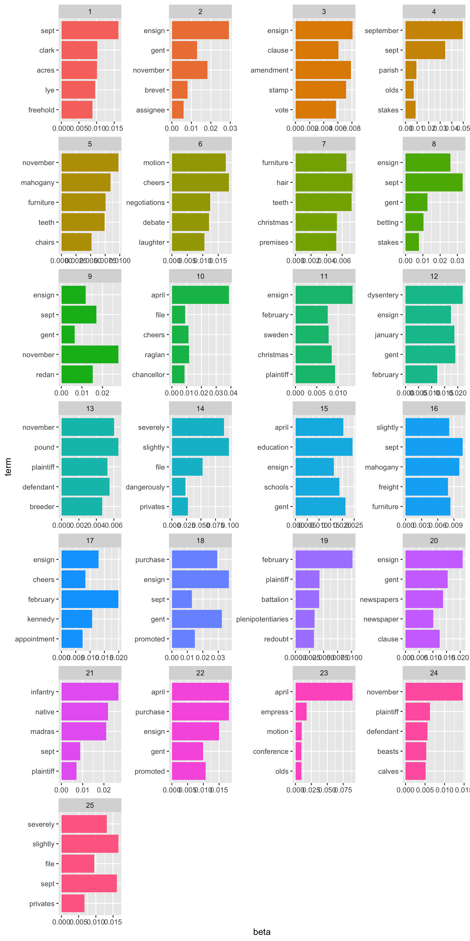
Figure 14.1: Sample Topics
You can also group the articles by their percentage of each ‘topic’, and use this to find common thread between them - for more on this, see here: https://www.tidytextmining.com/topicmodeling.html